Solving Inverse Problems with MCMC
Problem preface
You’re a detective, and you’re currently working to track down a notorious drug kingpin. If you can find his base-of-operations, you’ll be able to build a case against him.

You receive a tip that this individual is meeting someone at the city center in 20 mins. The center of the city is marked by a monument and surrounded by a large circular park, so you’ll have to walk. Can you make it in time? It is exactly 1 mile to the center, and you know you can walk a mile in 19.5 minutes. Therefore, it will take you 19.5 mins to reach the center, you can make it.
The forward problem
This is a forward problem, you know the parameters of the world and you are interested in predicting an outcome. Here, we know the distance we want to travel and the speed at which we can travel. From this, we’re able to predict the time it will take (outcome):
\[\begin{align} t &= d \cdot s \\ &= 19.5 \end{align}\]wherein $d$ is the 1 mile distance and $s$ is your walking speed.
You reach the park center and see the drug kingpin talking with another person! You strategically pick a place to sit nearby and fake-read a newspaper. You overhear him mention it took him 20 mins to walk to this location. From the information provided, do you know the location of the kingpin’s base-of-operation? It took them the about the same time to reach the same point, is this person is your neighbor?
The inverse problem
This is the inverse problem. We have observed an outcome (time it took to walk), and we want to infer a property of the world (starting location).
Complications with the inverse problem
So, can we tell if this person is our neighbor? No.
Very often, inverse problems are ill posed. We do not have enough information to completely solve the problem: we don’t know how fast they walk and, even if we did, the solution is not unique (discussed below).
If we want to find a solution to this incomplete problem, we will be required to leverage assumptions and prior knowledge. For example, let’s say we take an educated guess that, based on their build, this individual walks about the same speed as us. We formulate it mathematically by saying they walk a mile in $(19.5 \pm .5)$ minutes.
Solving the inverse problem with MCMC
We define the forward problem as
\[\begin{align} F(x_1, x_2, s) &= s \cdot \sqrt{x_1^2 + x_2^2} \\ &= t \end{align}\]where $(x_1, x_2)$ is a given starting location and $s$ is the walking speed. We can then propose (randomly guess) a set of candidate points and run them through the forward problem, we then see if the solution makes sense by comparing the result to our observation, 20 min. If the result matches our observation, we’ll save that candidate starting location as a plausible solution. We assume we are completely ignorant about their starting location, so we pull our random guesses from a uniform distribution across the entire city (2 miles x 2 miles).
We’ve already estimated this person walks about as fast as us. So, for each proposed starting location, we’ll also have to generate a walking speed and we’ll sample this from a Normal distribution.1
Lastly, we don’t know if it took them exactly 20 mins to walk. Typically, people tend to round times to give an number divisible by 5 in conversation (e.g. 12.2 minutes becomes 12 minutes), so we should incorporate this into our model. This is an “observational error”.2
We now have our full Bayesian model.
x1 ~ Uniform(-2, 2)         # sample starting location in x1
x2 ~ Uniform(-2, 2)         # sample starting location in x2
s ~ Normal(19.5, .5)        # sample walking speed
t = F(s, x1, x2)            # run forward problem to get predicted time
y ~ Normal(t, 3/2)          # predicted time considering observational error
To do anything useful with it we’ll need to leverage MCMC. For python, we have a few options at our disposal; I’ve chosen numpyro for this example and use the NUTS MCMC sampler.3
def model(obs):
    x1 = numpyro.sample('x1', dist.Uniform(-2, 2))
    x2 = numpyro.sample('x2', dist.Uniform(-2, 2))
    s = numpyro.sample('s', dist.Normal(19.5, .5))
    t = F(x1, x2, s)
    return numpyro.sample('obs', dist.Normal(t, 1.5), obs=obs)


kernel = NUTS(model)
mcmc = MCMC(kernel, NUM_WARMUP, NUM_SAMPLES)
mcmc.run(rng_key_, obs=np.array([20]))
mcmc.print_summary()
We run our model and we get the following results:
        mean       std    median      5.0%     95.0%     n_eff     r_hat
 S     19.48      0.50     19.48     18.68     20.32   8971.39      1.00
X1      0.00      0.73      0.00     -1.03      1.04   5148.41      1.00
X2     -0.02      0.73     -0.03     -1.05      1.02   5363.95      1.00
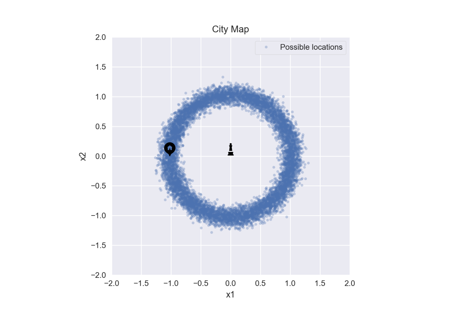
This says that the average inferred starting location is $(0,0)$ …basically the location we’re standing. This doesn’t make sense. Let’s look at the samples to understand this more.
Interpreting our results

Ah, this makes perfect sense. All possible locations are a ring with radius ~ 1 mile - if we average all of these we get the center of the ring, $(0,0)$.
Obtaining more information
Obviously, we still can’t tell if this person is our neighbor - they could live anywhere around this ring.
| I use this example because this really stresses the meat of your job as a data scientist (well, the meat of your job is cleaning data, but this is what gets you paid). Someone who runs a model and blindly trust whatever number is returned is likely to be mislead. Instead, you need a healthy dosage of extreme skepticism to dig though the model and find how it might be misleading you. Once you find what's wrong, you need to think about what piece(s) of information will help narrow the result. |
As you’re eavesdropping on this conversation, you notice they are holding a sandwich bag. You know this deli - it’s a popular local spot. The people in the immediate neighborhood go to it all the time, but it’s only a hole-in-the-wall so people further away don’t really know about it. However, if someone from that neighborhood moves across the city, they’ll still drive over to get their fix. This is useful information to us because it provides some information on the positional variables.
We fold this into our model by updating our prior guess on their starting location. We will assume a Laplacian distribution based on what we know about the deli.4
Our model is now:
x1 ~ Laplacian(-1.5, .1)    # sample starting location in x1
x2 ~ Laplacian(1, .1)       # sample starting location in x2
s ~ Normal(19.5, .5)        # sample walking speed
t = F(s, x1, x2)            # run forward problem to get predicted time
y ~ Normal(t, 3/2)          # predicted time considering observational error
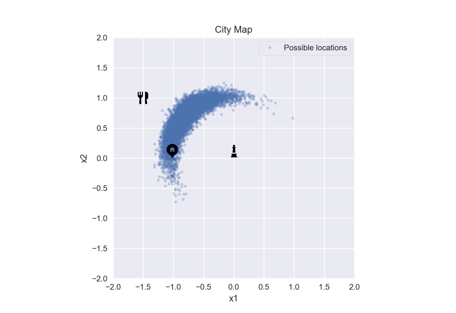
We run the model again we get the following samples:

Drawing conclusions
You can qualitatively tell that more information is needed to improve our model; but, for the sake of this example, we’ll stop here. What can we do with the results that we have?
What is the most probable location?
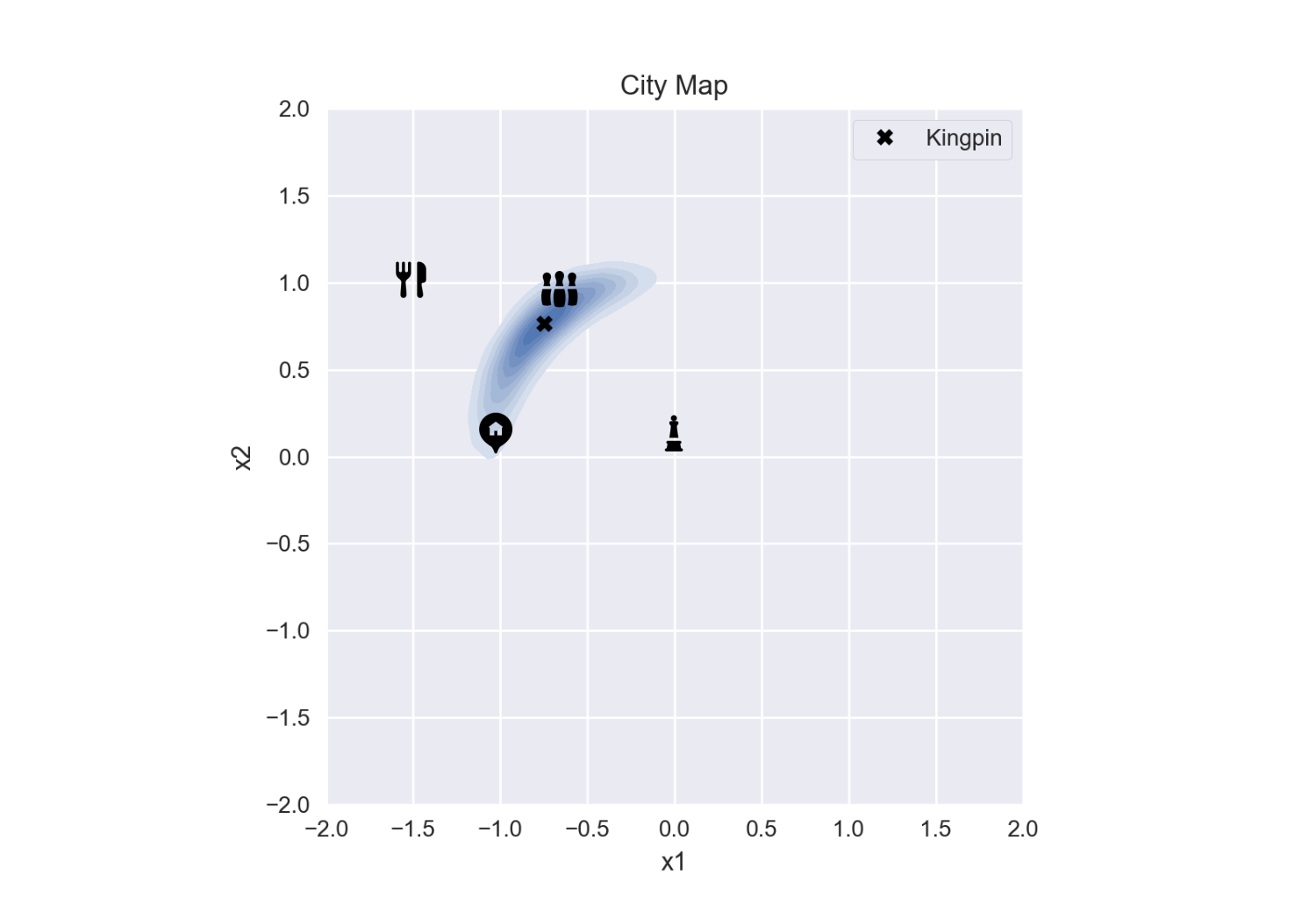
The most probable location is not the average of these samples (remember how that lead us astray in our first attempt?). Instead, we need to find the point with the highest density of accepted starting locations, the mode. To do this we’ll approximate the samplings as a pdf using a Gaussian kernel density estimation.5 We can then find the maximum point using gradient descent.
from scipy.optimize import minimize
from scipy.stats import gaussian_kde

kde = gaussian_kde(np.vstack([x1, x2]))
minimize(lambda x: -kde(x), [-1, 0])
x: array([-0.74703862, 0.76423531])
We have now identified the highest probable location of the kingpin based on our assumptions.

What is the probably they live near you?
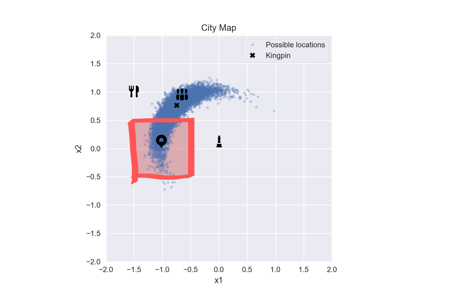
If we wanted to answer the original question: is this person is our neighbor? we can find the probability of this given our MCMC samples. We’ll define our neighborhood as $\pm 0.5$ miles around our house.

We can find this very easily using the samples obtained from our MCMC model. The probability is the number of samples inside our neighborhood, divided by the total number of samples.
P = np.mean((x1 < -.5) & (x1 > -1.5) & (x2 < .5) & (x2 > -.5))
print(f"Probability the kingpin is your neighbor: {100*P:.2f}%")
Probability the kingpin is your neighbor: 22.68%
Decision making
Lastly, how can we use this to inform our actions?
How much time should we spend looking for the base of operations in our neighborhood? Well, if we have 5 days to find him, we should only spend 22.68% of it in our neighborhood, or about 1 day and 3 hours.6
Final remarks
Hopefully this gives you an idea of how to leverage MCMC to solve inverse problems. You can view the full code on github.
References
-
If you ask “why a normal distribution” I strongly recommend this youtube video from Statistical Rethinking Winter 2019 Lecture 03 ↩
-
Let’s assume that 99.7% of people round to the nearest 5 baised on their watch-hand integer. e.g. 3 is rounded to 5 but 2.9 is rounded to 0. The 99.7 percentile is 2$\sigma$ so our standard dieviation is $3/2$ ↩
-
If you you want to know more about the NUTS MCMC sampler I strongly recommend this blog post on MCMC sampling methods ↩
-
This does a pretty good job reflecting the highest probability being near the mean, while supporting outliers (people who use to live in the neighborhood and have moved) ↩
-
Kernel density estimation is a way to estimate the probability density function (PDF) of a random variable in a non-parametric way ↩