What learning rate should I use?
One of the first questions you’ll ask yourself when starting to train a neural network is “what do I set the learning rate to?” Often the answer to this is one of those things in deep learning people lump into the “alchemy” category… Just because there really isn’t a one size-fits-all answer. Instead, it takes tinkering on the part of the researcher to find the most appropriate number for that given problem. This post tries to provide a little more intuition around picking appropriate values for your learning rates.
The shape of the loss surface, the optimizer, and your choice for learning rate will determine how fast (and if) you can converge to the target minimum.
\[w \leftarrow w - \eta \frac{d\mathcal{L}}{dw},\]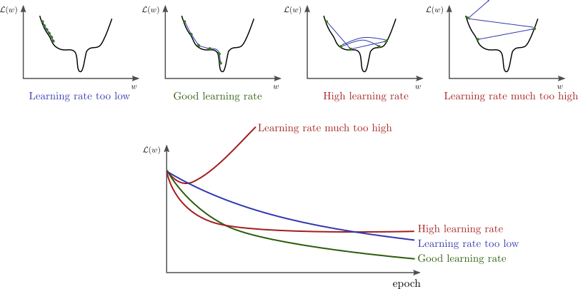
- A learning rate that is too low will take a long time to converge. This is especially true if there are a lot of saddle points in the loss-space. Along a saddle point, $d \mathcal{L} / dw$ will be close to zero in many directions. If the learning rate $\eta$ is also very low, it can slow down the learning substantially.
- A learning rate that is too high can “jump” over the best configurations
- A learning rate that is much too high can lead to divergence
Visualizing the loss surface
I’m a visual learner, and that can make it difficult to build intuition in a field like deep learning which is inherently high-dimensional and hard to visualize. Nevertheless, I’ve found it a useful exercise to seek out these illustrative descriptions. So how do you build a mental picture of things in high-dimensional space?
“To deal with hyper-planes in a fourteen dimensional space, visualize a 3D space and say ‘fourteen’ to yourself very loudly. Everyone does it.” – Geoffrey Hinton
I have found this work to be helpful in building up some intuition for understanding the neural network loss surfaces.
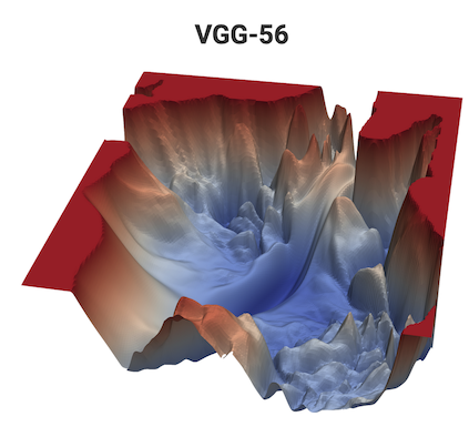
This is, of course, a 3D projection of a very high-dimensional function; it shouldn’t be believed blindly. Nevertheless, I think it’s helpful to hold this image in your mind for the discussion below.
Pick an optimizer
One of the choices you’ll make before picking a learning rate is “What optimizer to use?” I’m not going to dive into this. There’s already a wealth of good literature on the topic. Instead, I’ll just cite the links which I’ve found helpful.
- Why Momentum Really Works
- c231
- An overview of gradient descent optimization algorithms
- AdamW and Super-convergence is now the fastest way to train neural nets
For this post, I’ll only be talking about SGD. But, be aware that your choice of optimizer will also effect the learning rate you pick.
The connection between learning rate and batch size
Batch size is another one of those things you’ll set initially in your problem. Usually this doesn’t require too much thinking: you just increase the batch size until you get an OOM error on your GPU. But lets say you want to scale up and start doing distributed training.
When the minibatch size is multiplied by k, multiply the learning rate by k (All other hyperparameters are kept unchanged (weight decay, etc)
\[\begin{align*} w_{t+k} &= w_t - \eta \frac{1}{n}\sum_{j<k}\sum_{x\ni B} \nabla l(x, w_{t+j}) \\ \hat{w}_{t+k} &= w_t - \hat{\eta} \frac{1}{kn}\sum_{j<k}\sum_{x\ni B} \nabla l(x, w_{t+j}) \end{align*}\]With
\[\hat{\eta} = k\eta\]Let’s try this out. Pull down this simple cifar10 classifier and run it:
$ python cifar10.py

    Hyperparameters
    ---------------
    Batch size: 4
    learning rate: 0.001

loss: 0.823: 100%|###################################################| 10/10 [03:19<00:00, 19.90s/it]
Test Accuracy: 62.72%
We get ~63% accuracy, not bad for this little model. But this was pretty slow, it took about 20s/epoch on my Titian 1080ti. Lets bump up the batch size to 512 so it trains a bit faster.
$ python cifar10.py --batch-size 512 --lr .001

    Hyperparameters
    ---------------
    Batch size: 512
    learning rate: 0.001

loss: 2.293: 100%|###################################################| 10/10 [00:30<00:00,  3.10s/it]
Test Accuracy: 17.67%
Well… It trained faster, about 3s/epoch, but our accuracy plummeted. Let’s apply what we learned above. We increased our batch size by approximately 100, so let’s do the same to learning rate.
$ python cifar.py --batch-size 512 --lr .1

    Hyperparameters
    ---------------
    Batch size: 512
    learning rate: 0.1

loss: 0.888: 100%|###################################################| 10/10 [00:30<00:00,  3.09s/it]
Test Accuracy: 62.42%
And we’re back! In practice, it’s best to train with a lower learning rate initially and increment by a constant amount over ~5 epochs to improve stability. Check out this repo for a lr scheduler that does exactly that: pytorch-gradual-warmup-lr
Picking the best learning rate
Reduce learning rate on plateau
The most effective method I’ve found for managing learning rate is the approach of reducing the learning rate on plateau. This functionality or a similar functionality is built into all deep learning frameworks
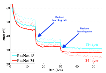
Every time the loss begins to plateau, the learning rate decreases by a set fraction. The belief is that the model has become caught in region similar to the “high learning rate” scenario shown at the start of this post (or visualized in the ‘chaotic’ landscape of the VGG-56 model above). Reducing the learning rate will allow the optimizer to more efficiently find the minimum in the loss surface. At this time, one might be concerned about converging to a local minimum. This is where building intuition from an illustrative representation can betray you, I encourage you to convince yourself of the discussion in the “Local minima in deep learning” section.
Use a learning-rate finder
The learning rate finder was first suggested by L. Smith and popularized by Jeremy Howard in Deep Learning : Lesson 2 2018. There are lots of great references on how this works but they usually stop short of hand-wavy justifications. If you want some convincing of this method, this is a simple implementation on a linear regression problem, followed by a theoretical justification.
Toy Example
We want to fit a simple line $y=wx$ with $w=2.5$. Of course when we start, we don’t know $w$.
We randomly select a value for $w$ and we have some loss associated with that:
\[\mathcal{L} = \frac{1}{N}\sum_i^N (y_i-wx_i)^2\]If we step through values for $w$ systematically, we can built out a plot of the loss surface. Because this in 1D we can easily visualize it, exactly.
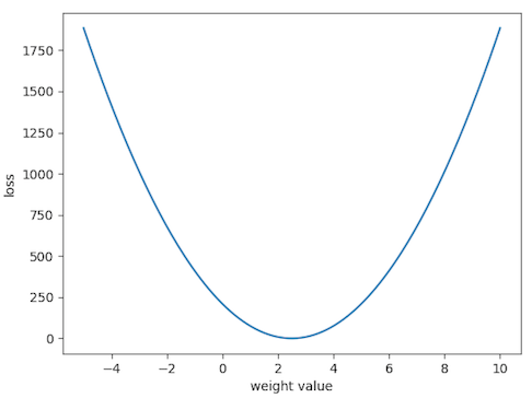
As we expect, we see a minimum for $\mathcal{L}$ when $w=2.5$. In practice, we wouldn’t want to generate this plot. The problem would quickly become intractable if you were to search over every permutation of parameters. Instead, we want to use gradient decent to iteratively converge on the correct $w$.
\[w \leftarrow w - \eta \frac{d\mathcal{L}}{dw},\]To find the optimal learning rate, $\eta$, we randomly select a value for $w$. Lets say we pick “8”. For $w=8$ there’s a loss associated with that: ~1e3, given by the above graph.
We then take a tiny step, which is determined by the smallest learning rate we want to use (min_lr in the example implementation code), and recalculate our loss. We didn’t move very far, so our loss is about the same, ~1e3.
We keep doing that, slowly increasing the $\eta$ each time. Eventually, we’ll find a point where we start moving down the loss function faster. We can see this if we plot our loss vs the lr during this exploration.
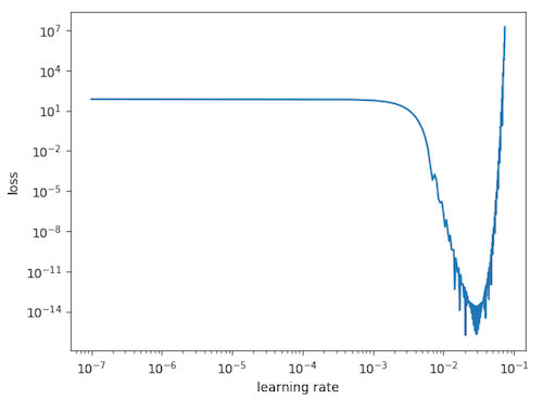
We’re interested in the region where we’re moving down the loss function the fastest, i.e. the region of the largest change in loss for a given learning rate. So, we select ~1e-2 as our optimal learning rate.
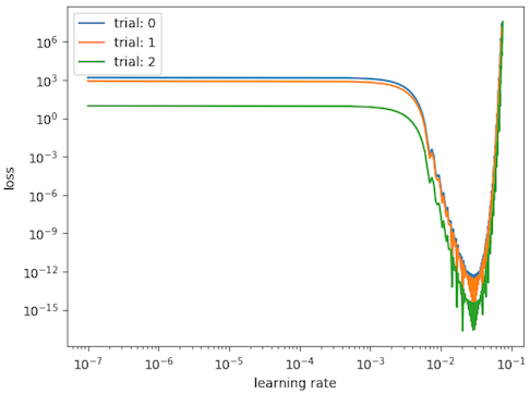
We can repeat this experiment multiple times. Even though we initialize our $w$ at different points on the loss surface, we see the optimal learning rate works out to be the same.
Theoretical justification
We can confirm this number analytically with the mechanics outlined by Goodfellow 4.3.1. We start by taking a Taylor expansion of the loss function about the point $w_i$. This $w_i$ is our arbitrary initial point.
\[\mathcal{L}(w) \approx \mathcal{L}(w_i) + (w-w_i)\mathcal{L}'\Bigr|_{w=w_i} + \frac{1}{2}(w-w_i)^2 \mathcal{L}''\Bigr|_{w=w_i}\]We can evaluate this function at an arbitrary distance away from our initial point:
\[w=w_i + \eta\mathcal{L}'\Bigr|_{w=w_i}.\]Such that we’ve defined this distance as a function of our learning rate $\eta$.
Now, we know the loss will be at a minimum when $\mathcal{L’(w)}=0$. Let’s call this final target location $w_f$. Our optimal learning rate, $\eta^*$, will then be one where we can take one single step to go from $w_i$ to $w_f$.
\[\begin{align*} \frac{d}{dw}\mathcal{L}(w)\Bigr|_{w=w_f} &\approx \frac{d}{dw}\left [ \mathcal{L}(w_i) + (w-w_i)\mathcal{L}'\Bigr|_{w=w_i} + \frac{1}{2}(w-w_i)^2 \mathcal{L}''\Bigr|_{w=w_i} \right ]_{w=w_f} \\ &\approx \mathcal{L}'\Bigr|_{w=w_i} + (w_f - w_i)\mathcal{L}''\Bigr|_{w=w_i} \\ &= 0 \\ \end{align*}\]Solving for our optimal learning rate, we get the following relation:
\[\eta^* = \frac{1}{\mathcal{L}''\Bigr|_{w=w_i}}\]Taking the second derivative of our loss function
\[\begin{align*} \frac{d^2}{dw^2}\mathcal{L} \Bigr|_{w=w_i} &= \frac{1}{N}\sum_i^N \frac{d^2}{dw^2} (y_i-wx_i)^2 \\ &= \frac{1}{N} \sum_{i}^{N} x_i^2 \frac{d^2}{dw^2} (w_f - w)^2 \\ &= \frac{1}{N} \sum_{i}^{N} x_i^2 w_f \\ \end{align*}\]we confirm that the optimal learning rate will be independent of $w_i$.
Substituting in our values above: $w_f=2.5$ and $x$ to be 100 points in the range $[0, 10)$. We get our optimal learning rate to be:
\[\eta* = 1.2\mathrm{e}{-2}\]This will get us to the bottom in one step. And sure enough, if we examine our derived value on the loss v lr plots above, we see a minimum at this location - showing that we’ve reached the bottom on the loss surface.
Now, in practice (e.g. the VGG-56 loss surface, above), the Taylor series is unlikely to remain accurate for large $\eta$ [Goodfellow 4.3.1]. So, we pick a more conservative value to avoid over shooting our minima. 1e-2 is a pretty good choice, which is encouraged by our learning-rate finder.
Additional Notes
Other methods for controlling learning rate
- Cyclical Learning Rates
- Transfer learning and Freezing Layers
- Differential Learning Rates
Local minima in deep learning
Difficulty in convergence during neural network training is due to traversing saddle points, not becoming stuck in local minima. In high-dimensional problems, saddle points are surrounded by “high-error plateaus that can dramatically slow down learning”. This behavior gives the impression of the existence of a local minimum.
This was very well addressed on the Data Science Stack Exchange by David Masip. I’ll include the justification here in case the link dies.
The condition for a point on the loss-surface to be a minimum is that the Hessian matrix, $\mathcal{H}$, is positive for every value in it. Because the Hessian is symmetric, we can represent it as a diagonalized matrix:
\[\mathcal{H} = \frac{d^2 \mathcal{L}}{d w_i d w_j} = \begin{bmatrix} w_{1} & & \\ & \ddots & \\ & & w_{n} \end{bmatrix}\]Therefore, the probability the point is a minimum is the probability that every value in the Hessian is positive:
\[P(w_1 > 0, \dots, w_n > 0) = P(w_1 > 0)\cdot \cdots \cdot P(w_n > 0) = \frac{1}{2^n}\]For a point to be a maximum, we assume the same thing except that every value in the Hessian is negative. If a point is not a minimum and it is not a maximum, it must be a saddle point. Trivially, we can see the probability of this is very likely:
\[P({\rm saddle}) = 1 - P({\rm maximum}) - P({\rm minimum}) = 1 - \frac{1}{2^n} - \frac{1}{2^n} = 1 - \frac{1}{2^{n-1}}\]Such that $P({\rm saddle}) \approx 1$ for large n.