Line-VISAR Analysis
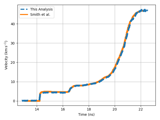
This post outlines the FFT analysis routine for line-VISAR data. The code implementing this routine can be found here: https://github.com/bdhammel/line-visar-analysis. I benchmark this script against the published data by Smith et al. on the ramp compression of diamond to 5 TPa.
Analysis
As stated in my previous post on Line-VISAR Theory, the fringe shift recorded is directly proportional to the velocity of the target. It is, therefore, the goal of the analysis routine to extract the percentage fringe shift at a given location and time. Several methods exist for accomplishing this. However, the Fourier transform method (described here), first proposed by Takeda et al, has been determined to be the most accurate [Celliers].
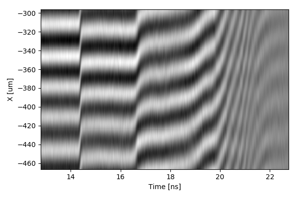
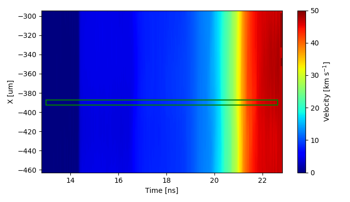
The raw data (shown above) is typically cropped to analyze the region of planar shock breakout (enclosed in the red rectangle, with reference fringes enclosed in green).

This image can be described mathematically using the equation for intensity, $I(x, t)$, with $ b(x,t ) = I_1+I_2 $ being the background and $ a(x,t) = 2\mathbf{E_1}\mathbf{E_2} $ describing the intensity of the fringes. $\phi (x,t)$ represents the phase of the fringes and $2\pi f_{0}x + \delta_{0} $ describes the linear phase ramp of the background fringe pattern. The goal is to find $ \phi (x,t) $, which is directly proportional to the velocity of the target. Rewriting the intensity equation in terms of its complex components yields:
\[\begin{align} && f(x,t) &= b(x,t)+c(x,t)e^{i2\pi f_{0}x} + c^*(x,t)e^{-i2\pi f_{0}x },& \\ \text{with} && c(x,t) &= \frac{1}{2}a(x,t)e^{i\delta_{0}}e^{i\phi (x,t)}. \end{align}\]A Fourier transform is applied to the data at each point-in-time
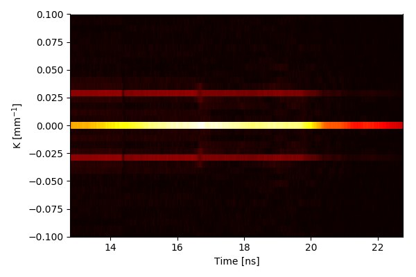
the background, $b(x,t)$, can then be removed by filtering specific frequencies (such that the pixel values are set to zero):
\[\require{cancel} \begin{align*} F(f,t) &= B(f,t)+\int_{ -\infty }^{\infty} c(x,t) e^{i2\pi f_{0}x}e^{-ifx} \; dx + \int_{-\infty }^{\infty}c^*(x,t)e^{-i2\pi f_{0}x }e^{-ifx} \; dx \\[1.5ex] &=B(f,t)+\int_{-\infty }^{\infty}c(x,t)e^{i2\pi (f_{0}-f) x} \; dx + \int_{-\infty }^{\infty}c^*(x,t)e^{-i2\pi (f_{0} +f )x} \;dx \\[1.5ex] &=\cancelto{0}{B(f,t)}+\cancelto{0}{C^*(f+f_0,t)}+C(f-f_0,t). \end{align*}\]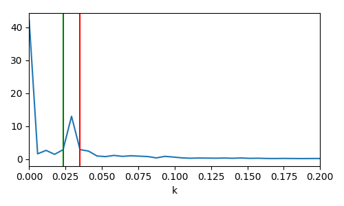
Applying an inverse Fourier transform:
\[\begin{align} d(x,t) &= \int_{-\infty}^{\infty}C(f-f_0,t)e^{ixf} \; df \nonumber \\ &= \int_{-\infty}^{\infty}C(f-f_0,t) \left ( \cos(xf) + i\sin(xf) \right ) \; df \label{eqn:ifft} \\ &=c(x,t)e^{2\pi i f_0x} \label{eqn:filtered} \end{align}\]results in the filterd image.
The above image has both a real and imaginary valued function. Where
\[\begin{align} && \operatorname{Re} [d(x,t) ] &\propto \sin( \phi (x,t) + 2\pi f_0 x + \delta_0) \label{eqn:re},& \\ \text{and} && \operatorname{Im} [d(x,t) ] &\propto \cos( \phi (x,t) + 2\pi f_0x + \delta_0) \label{eqn:im}, \end{align}\]are $\pi/2$ out of phase. Taking the $\arctan$ of the ratio allows the phase, $\phi (x,t) + 2\pi f_0x + \delta_0$, to be extracted:
\[\begin{equation*} W( \phi (x,t) + 2\pi f_0x + \delta_0) = \arctan\left ( \frac{\operatorname{Re} [d(x,t) ]}{\operatorname{Im} [d(x,t) ]} \right ). \end{equation*}\]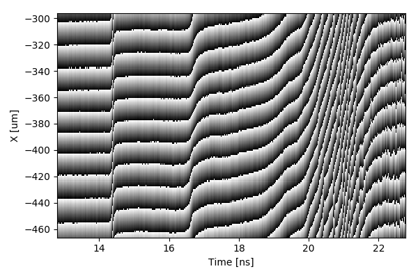
The resulting function $W$ has discontinuities representing $\pi$ shifts as the $\arctan$ moves through full rotations. The velocity signal can be constructed by removing these discontinuites and scaling the values by the proportionality factor VPF. The programatic method for reconstructing the velocity trace from the time dependent values in the wrapped phase can be accomplished via the psudocode bellow:
_max_dphase = np.pi/2. - _threshold
_min_dphase = -1 * _max_dphase
vpf = 1.998 # velocity per fringe shift for a given etalon

for row in image:
    for column_idx in lenth_of_row):
        dphase = row[i] - row[i-1]
        if dphase < _min_dphase:
            dphase += np.pi
        elif dphase > _max_dphase:
            dphase -= np.pi
        v += dphase * vpf / (2*np.pi)
References
- R. F. Smith et al., “Ramp compression of diamond to five terapascals,” Nature, vol. 511, pp. 330–333, jul 2014.
- L. Barker and R. Hollenbach, “Laser interferometer for measuring high velocities of any reflecting surface,” Journal of Applied Physics, vol. 43, pp. 4669–4675, November 1972.
- Y. B. Zel’dovich and Y. P. Raizer, Physics of Shock Waves and High-Temperature Hydrodynamic Phenomena. Dover, 2002.
- P. Celliers et al., “Line-imaging velocimeter for shock diagnostics at the OMEGA laser facility,” Review of Scientific Instruments, vol. 75, November 2004.
- D. J. Robinson, “Optically relayed push-pull velocity interferometry resolved in time and position,” Master’s thesis, Washington State University, 2005.
- G. Fowles, Introduction to Modern Optics. Dover, 1989.
- M. Takeda et al., “Fourier-transform method of fringe-pattern analysis for computer-based topography and interferometry,” Journal of the Optical Society of America, vol. 72, pp. 156–160, January 1983.
- D. H. Dolan, “Foundations of VISAR analysis.,” tech. rep., Sandia National Laboratories, Jun 2006.