Line-VISAR Theory
Velocity Interferometer System for Any Reflector
The Velocity Interferometer System for Any Reflector (VISAR) [Barker] is a principal diagnostic in dynamic compression research. The VISAR works by analyzing the Doppler shift of a pulse of light which has been reflected off of a moving surface (e.g. the back surface of a sample as a shock wave emerges). By examining the frequency change of the light, the velocity of the moving surface can be found, allowing the material properties (such as the pressure) to be inferred from the application of classical mechanics including the laws of mass, momentum, and energy conservation, as well as knowledge of the initial physical condition of the target material [Zel’dovich].
VISAR Theory of Operation
The frequency change in the VISAR’s probe beam, due to a moving target with velocity $v(t)$, is governed by the Doppler equation,
\[\begin{equation} \lambda (t)=\lambda_{0}\left( 1-\frac{2v(t)}{c} \right ). \end{equation}\]The Doppler shifted light is passed through a Mach-Zehnder interferometer, where one leg of the interferometer is delayed by placing an etalon in the ray path. The recombination of the two legs generates a fringe comb pattern overlaid on the image of the target surface. A line-out of this is then recorded using a white-light streak camera. The result is an image with spatial and temporal information of the target, as seen in in the below figure [smith].
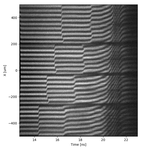
The shift in the fringes is directly proportional to the velocity of the object that the light was reflected from,
\[v \propto \left \{ \text{fringe shift}\right \}.\]The proportionality constant of this relation is found by starting with the equation of a plane wave,
\[\begin{equation} \mathbf{E}=\mathbf{E_0}e^{i \left ( \mathbf{k}\cdot\mathbf{r} - \omega t + \delta \right )}, \end{equation}\]and solving for the superposition of the beams from both legs of the interferometer at the detector surface [Fowles],
\[\begin{align} I &\equiv \left | \mathbf{E} \right | \nonumber \\ &= \mathbf{E}\cdot\mathbf{E}^* \nonumber \\ &=\left(\mathbf{E_1}+\mathbf{E_2}\right) \cdot \left(\mathbf{E_1^*}+\mathbf{E_2^*}\right) \nonumber \\ %&=\left |\mathbf{E_1}\right|^2+ \left|\mathbf{E_2} \right|^2 + \mathbf{E_{1,0}}\cdot \mathbf{E_{2,0}} \left ( \frac{e^{i \left ( \left (\mathbf{k_1} - \mathbf{k_1} \right ) \cdot\mathbf{r} - \omega_1 t + \delta\right )} + e^{-i \left ( \left (\mathbf{k_1} - \mathbf{k_2}\right ) \cdot\mathbf{r} - \omega_2 t + \delta\right )} }{2} \right ) \nonumber \\ &=I_1+I_2 + 2\mathbf{E_{1,0}}\cdot \mathbf{E_{2,0}}\cos \theta. \end{align}\]The $2\mathbf{E_{1,0}}\cdot \mathbf{E_{2,0}}\cos \theta$ term describes the resulting interference. With
\[\theta = \mathbf{k_1 \cdot r_1} - \mathbf{k_2 \cdot r_2} - \omega_1 t_1 + \omega_2 t_2 + \delta_1 + \delta_2\]and can be simplified as a time dependent phase with a constant offset, $\phi (t) + \delta_{0}$. Wherein
\[\begin{equation} \phi(t) = 2\pi F(t) \end{equation}\]such that $F(t)$ is the fractional fringe shift, proportional to the velocity of the target. The intensities can then be grouped into a background term, $b(t)$, and amplitude of the interference, $a(t)$, for a general form:
\[\begin{equation} I(t) = b(t)+a(t)\cos[\phi (t) + \delta_{0}]. \end{equation}\]Considering the 1D case, with the optical system in perfect alignment such that all interferometer optic surfaces are perfectly parallel, the interference of two beams, $\mathbf{E_1}$ and $\mathbf{E_2}$, will be determined by the time delay,
\[\begin{equation} \tau = \frac{2h}{c}(n-1). \end{equation}\]In which $\tau$ is a function of the etalon (thickness $h$) placed in the path of one leg of the interferometer. The Doppler-shifted frequency of the reference beam and the time delayed beam can then be used to find $\theta$.
What this $\tau$ ends up meaning is that we’ll observe the Doppler-shifted frequency of the probe beam at two different times of its history. Because the position of the reflector has changed during these two times, the phase will have propagated a different distance, $r_1$ and $r_2$, for the interfering rays, $E_1$ and $E_2$. We rewrite the phase, $\psi$, as if the time of propagation, $t$, is the same - allowing us to drop the term $\omega t$ and considering the phase propagation as a function of distance, $r$:[Dolan]
\[\begin{align} && \psi (t') &= \mathbf{k}(t')\cdot \mathbf{r}(t') \\ \text{such that} && \phi &= \psi_1 - \psi_2. \end{align}\]To simplify the problem, we can assume this distance, $r$, is the distance the probe beam takes to the reflector plus the distance it takes from the reflector to the detector. Illustratively put:
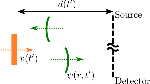
Because we will be making a relative comparison, we can drop terms which are consistent between the two electric fields. Thus, the distance from the source-to-the-reflector and the distance from the reflector-to-the-detector is assumed to be equal, and reduced to be the total distance that the reflector will move during the detection time, $T$:
\[\begin{align} && d(t') &= \int_{t'}^T v(t) dt \\ \text{and} && r(t') &= 2d(t'). \end{align}\]During the propagation of the probe from the source-to-the-reflector, the wavelength of the light is the initial wavelength generated by the source, $k = \frac{2\pi}{\lambda_0}$. However, on the return path, the wavelength has now shifted, determined by the Doppler effect:
\[k(t') = \frac{2\pi c}{\lambda_0} \left ( \frac{1}{c-2v(t')} \right )\]The interference term, $\phi$, can now be expressed in the following way:
\[\begin{align*} \phi(t) &= \mathbf{k_1 r_1} - \mathbf{k_2 r_2} \\ &= k(t' - \tau) r(t' - \tau) - k(t') r(t') \\ &= \left \{ k(t' - \tau) + k_0 \right \} d(t' - \tau) - \left \{ k(t') + k_0 \right \} d(t') \\ \end{align*}\]Substituting in the definition for $k$ and assuming that $v(t’) \ll c$ leads to the expression:
\[\begin{align*} \phi(t) &= \frac{2\pi}{\lambda_0} \left \{ d(t'-\tau) - d(t') + c\frac{d(t'-\tau)}{c-2v(t'-\tau)} + c\frac{d(t')}{c-2v(t')}\right \} \frac{\tau}{\tau} \\ &\rightarrow \frac{2\pi \tau}{\lambda_0} 2 v(t') \end{align*}\]Allowing us to solve for $F(t)$ to get a resulting a Velocity Per Fringe (VPF) shift of:
\[\begin{equation} {\rm VPF} \equiv \frac{v(\tau)}{F(t)} = \frac{\lambda_0}{2\tau}. \end{equation}\]Extending this formalism to all space, and taking into consideration the imaging properties of the line-VISAR system, the function of intensity takes on a form dependent on $x$ and $t$,
\[\begin{equation} I(x,t) = b(x,t)+a(x,t)\cos[\phi (x,t)+2\pi f_{0}x + \delta_{0} ]. \end{equation}\]The equations for VPF and $\tau$ are then adjusted to account for dispersion of light in the etalon and the shift in the image location due to the etalon’s index of refraction:
\[\begin{align} {\rm VPF} &= \frac{\lambda_0}{2\tau(1+\delta)}, \\ \tau &= \frac{2h}{c}(n-1/n). \end{align}\]Simulated VISAR data
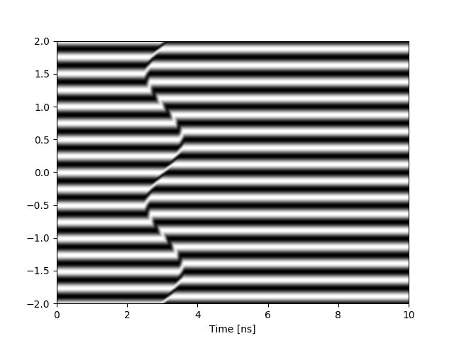
Using this mathematical procedure, we can then generate synthetic VISAR data for a given velocity profile. Please visit my GitHub repo on Simulated Line-Visar data
References
- R. F. Smith et al., “Ramp compression of diamond to five terapascals,” Nature, vol. 511, pp. 330–333, jul 2014.
- L. Barker and R. Hollenbach, “Laser interferometer for measuring high velocities of any reflecting surface,” Journal of Applied Physics, vol. 43, pp. 4669–4675, November 1972.
- Y. B. Zel’dovich and Y. P. Raizer, Physics of Shock Waves and High-Temperature Hydrodynamic Phenomena. Dover, 2002.
- P. Celliers et al., “Line-imaging velocimeter for shock diagnostics at the OMEGA laser facility,” Review of Scientific Instruments, vol. 75, November 2004.
- D. J. Robinson, “Optically relayed push-pull velocity interferometry resolved in time and position,” Master’s thesis, Washington State University, 2005.
- G. Fowles, Introduction to Modern Optics. Dover, 1989.
- M. Takeda et al., “Fourier-transform method of fringe-pattern analysis for computer-based topography and interferometry,” Journal of the Optical Society of America, vol. 72, pp. 156–160, January 1983.
- D. H. Dolan, “Foundations of VISAR analysis.,” tech. rep., Sandia National Laboratories, Jun 2006.