Maximum Likelihood Estimation and Maximum A Posterior Estimation
What is the difference between MLE and MAP?
Maximum likelihood is a special case of Maximum A Posterior estimation. To be specific, MLE is what you get when you do MAP estimation using a uniform prior. Both methods come about when we want to answer a question of the form: “What is the probability of scenario $Y$ given some data, $X$ i.e. $P(Y|X)$.
A question of this form is commonly answered using Bayes’ Law.
\[\underbrace{P(Y|X)}_{\rm posterior} = \frac{\overbrace{P(X|Y)}^{\rm likelihood} \overbrace{P(Y)}^{\rm prior}}{\underbrace{P(X)}_\text{probability of seeing the data}}.\]MLE
If we’re doing Maximum Likelihood Estimation, we do not consider prior information (this is another way of saying “we have a uniform prior”) [K. Murphy 5.3]. In this case, the above equation reduces to
In this scenario, we can fit a statistical model to correctly predict the posterior, $P(Y|X)$, by maximizing the likelihood, $P(X|Y)$. Hence “Maximum Likelihood Estimation.”
MAP
If we know something about the probability of $Y$, we can incorporate it into the equation in the form of the prior, $P(Y)$. In This case, Bayes’ laws has it’s original form.
We then find the posterior by taking into account the likelihood and our prior belief about $Y$. Hence “Maximum A Posterior”.
Using MLE or MAP estimation to answer a question
Let’s say you have a barrel of apples that are all different sizes. You pick an apple at random, and you want to know its weight. Unfortunately, all you have is a broken scale.

For the sake of this example, lets say you know the scale returns the weight of the object with an error of +/- a standard deviation of 10g (later, we’ll talk about what happens when you don’t know the error). We can describe this mathematically as:
\[{\rm measurment} = {\rm weight} + \mathcal{N}(0, 10g)\]Let’s also say we can weigh the apple as many times as we want, so we’ll weigh it 100 times.
We can look at our measurements by plotting them with a histogram
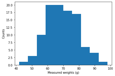
Now, with this many data points we could just take the average and be done with it
\[\begin{align} \mu &= \frac{1}{N} \sum_i^N x_i \\ {\rm SE} &= \frac{\sigma}{\sqrt{N}} \end{align}\]The weight of the apple is (69.62 +/- 1.03) g
If the $\sqrt{N}$ doesnt look familiar, this is the “standard error”
No surprises, nothing fancy.
If you find yourself asking “Why are we doing this extra work when we could just take the average”, remember that this only applies for this special case. It’s important to remember, MLE and MAP will give us the most probable value. For a normal distribution, this happens to be the mean. So, we will use this to check our work, but they are not equivalent.
- MLE = ‘mode’ (or ‘most probable value’) of the posterior PDF [E. Jaynes 6.11.1]
- mean = expected value from samples
Maximum Likelihood Estimation using a grid approximation
Just to reiterate: Our end goal is to find the weight of the apple, given the data we have. To formulate it in a Bayesian way: We’ll ask what is the probability of the apple having weight, $w$, given the measurements we took, $X$. And, because were formulating this in a Bayesian way, we use Bayes’ Law to find the answer:
\[P(w|X) = \frac{P(X|w)P(w)}{P(X)}\]If we make no assumptions about the initial weight of our apple, then we can drop $P(w)$ [K. Murphy 5.3]. We’ll say all sizes of apples are equally likely (we’ll revisit this assumption in the MAP approximation).
Furthermore, we’ll drop $P(X)$ - the probability of seeing our data. This is a normalization constant and will be important if we do want to know the probabilities of apple weights. But, for right now, our end goal is to only to find the most probable weight. P(X) is independent of $w$, so we can drop it if we’re doing relative comparisons [K. Murphy 5.3.2].
This leaves us with $P(X|w)$, our likelihood, as in, what is the likelihood that we would see the data, $X$, given an apple of weight $w$. If we maximize this, we maximize the probability that we will guess the right weight.
Enter the grid approximation:
The grid approximation is probably the dumbest (simplest) way to do this. Basically, we’ll systematically step through different weight guesses, and compare what it would look like if this hypothetical weight were to generate data. We’ll compare this hypothetical data to our real data and pick the one the matches the best.
To put this illustratively:
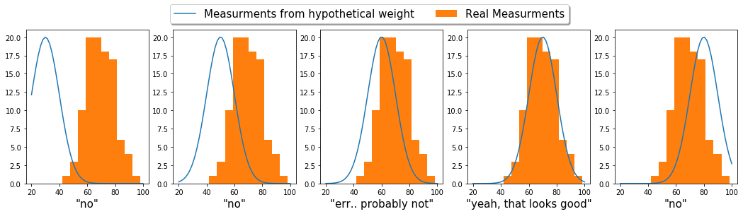
To formulate this mathematically:
For each of these guesses, we’re asking “what is the probability that the data we have, came from the distribution that our weight guess would generate”. Because each measurement is independent from another, we can break the above equation down into finding the probability on a per measurement basis
\[P(X|w) = \prod_{i}^{N} p(x_i | w)\]So, if we multiply the probability that we would see each individual data point - given our weight guess - then we can find one number comparing our weight guess to all of our data. We can then plot this:
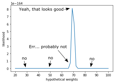
There you have it, we see a peak in the likelihood right around the weight of the apple.
But, you’ll notice that the units on the y-axis are in the range of 1e-164. This is because we took the product of a whole bunch of numbers less that 1. If we were to collect even more data, we would end up fighting numerical instabilities because we just cannot represent numbers that small on the computer. To make life computationally easier, we’ll use the logarithm trick [Murphy 3.5.3].
\[\begin{align} \log P(X|w) &= \log \prod_{i}^{N} p(x_i | w) \\ &= \sum_{i}^{N} \log p(d_i | w) \end{align}\]This is the log likelihood. We can do this because the likelihood is a monotonically increasing function
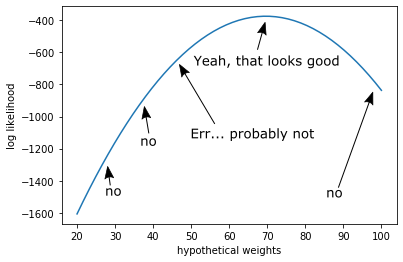
These numbers are much more reasonable, and our peak is guaranteed in the same place.
The weight of the apple is (69.39 +/- 1.03) g
In this case our standard error is the same, because $\sigma$ is known.
To implement this in code
Implementing this in code is very simple. The python snipped below accomplishes what we want to do.
from scipy.stats import norm
import numpy as np

weight_grid = np.linspace(0, 100)

likelihoods = [
  np.sum(norm(weight_guess, 10).logpdf(DATA))
  for weight_guess in weight_grid
]
weight = weight_grid[np.argmax(likelihoods)]
MLE grid approximation for multiple parameters
Now lets say we don’t know the error of the scale. We know that its additive random normal, but we don’t know what the standard deviation is
\[{\rm measurment} = {\rm weight} + \mathcal{N}(0, \sigma)\]We can use the exact same mechanics, but now we need to consider a new degree of freedom.
In other words, we want to find the mostly likely weight of the apple and the most likely error of the scale
\[P(w, \sigma |X) \propto P(X|w, \sigma)\]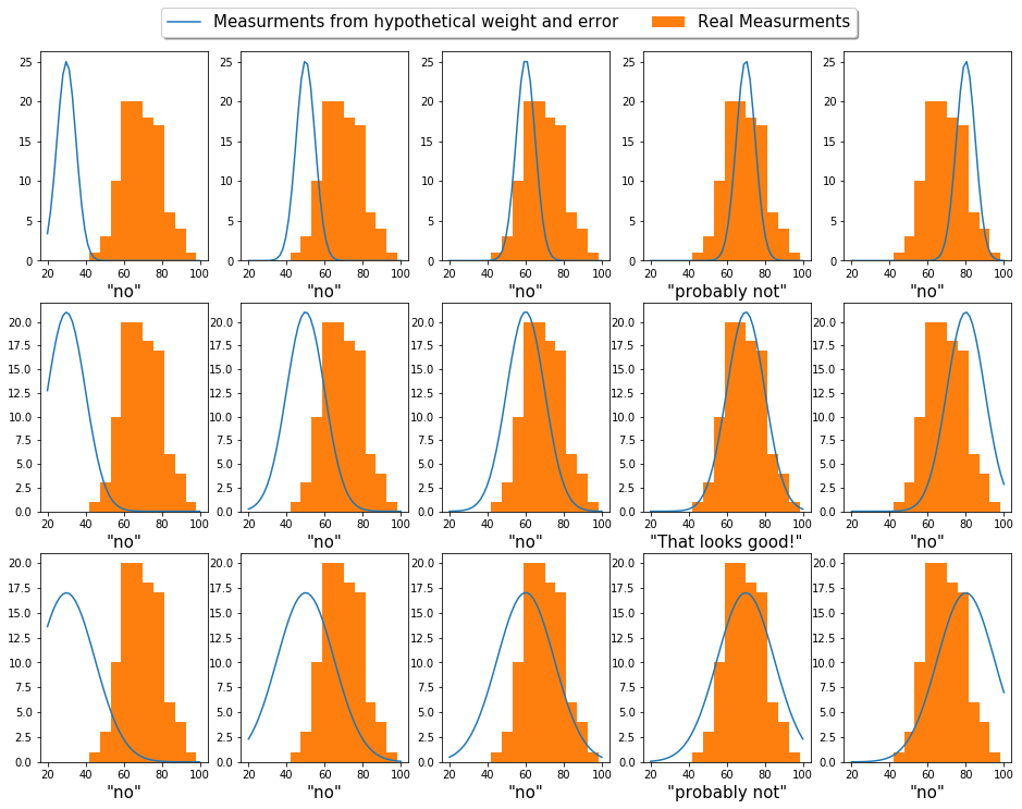
Comparing log likelihoods like we did above, we come out with a 2D heat map
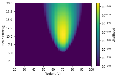
The maximum point will then give us both our value for the apple’s weight and the error in the scale.
The weight of the apple is (69.39 +/- .97) g
Maximum A Posterior with a grid approximation
In the above examples we made the assumption that all apple weights were equally likely. This simplified Bayes’ law so that we only needed to maximize the likelihood
\[P(w, \sigma|X) \propto P(X|w, \sigma)\]However, not knowing anything about apples isn’t really true. We know an apple probably isn’t as small as 10g, and probably not as big as 500g. In fact, a quick internet search will tell us that the average apple is between 70-100g. So, we can use this information to our advantage, and we encode it into our problem in the form of the prior.
\[P(w, \sigma|X) \propto P(X|w, \sigma)P(w, \sigma)\]By recognizing that weight is independent of scale error, we can simplify things a bit. So we split our prior up [R. McElreath 4.3.2]
\[P(w, \sigma) = P(w)P(\sigma)\]Like we just saw, an apple is around 70-100g so maybe we’d pick the prior
\[P(w) = \mathcal{N}(85, 40)\]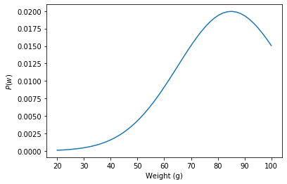
Likewise, we can pick a prior for our scale error. We’re going to assume that broken scale is more likely to be a little wrong as opposed to very wrong
\[P(\sigma) = {\rm Inv{-}Gamma}(.05)\]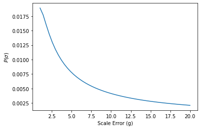
With these two together, we build up a grid of our prior using the same grid discretization steps as our likelihood. We then weight our likelihood with this prior via element-wise multiplication.
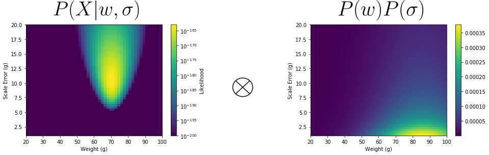
From this, we obtain our Posterior.
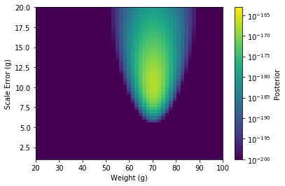
The weight of the apple is (69.39 +/- .97) g
In this example, the answer we get from the MAP method is almost equivalent to our answer from MLE. This is because we have so many data points that it dominates any prior information [Murphy 3.2.3]. But I encourage you to play with the example code at the bottom of this post to explore when each method is the most appropriate.
Example code
Play around with the code and try to answer the following questions
- How sensitive is the MAP measurement to the choice of prior?
- How sensitive is the MLE and MAP answer to the grid size?
A final note
I used standard error for reporting our prediction confidence; however, this is not a particular Bayesian thing to do. I do it to draw the comparison with taking the average and to check our work. In practice, you would not seek a point-estimate of your Posterior (i.e. the maximum). Instead, you would keep denominator in Bayes’ Law so that the values in the Posterior are appropriately normalized and can be interpreted as a probability. But, how to do this will have to wait until a future blog post.