Yet another post on backprop
Anatomy of a Neural Network
This seems to be the most common illustration of a neural network.
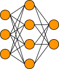
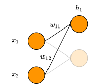
In this diagram, the edges of the graph are the network weights and the nodes are the neurons. That is,
Visualizing this network as a computational graph is a different representation, but it describes the same behaviors. However, this visualization will make it much easier to understand the mechanics of back propagation [Goodfellow, s6.5.1].
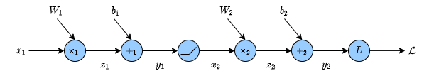
Here, the edges are data (e.g. input data, weights, biases, intermediate results, etc) and the nodes are computational operations (e.g. dot product, relu, convolution, loss function). This is the visualization of a network you would get if you were to export a pytorch model and visualize it in netron, or inspect the static graph of a tensorflow model.
Back Propagation
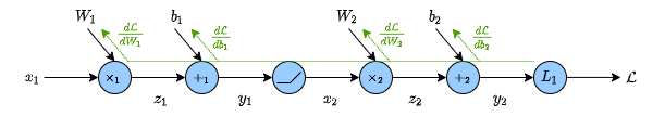
Looking at the graph, we said the edges (connection) were data and the nodes (circles) were operations. In the forward direction these edges are our intermediate results, in the backwards direction these edges are our gradients. (For the sake of simplicity lets assume all values are scalars, at this time).
We want to update our model’s weights, $W$ and $b$, based on how right or how wrong our prediction is. To quantify how far off from our target we are, we’ll use the ${\rm L}_1$-Loss function (i.e. the absolute value of the difference).
\[L_1(y,t) = \sum_i |y_i-t_i|\]with $y$ being our prediction and $t$ being our target value.
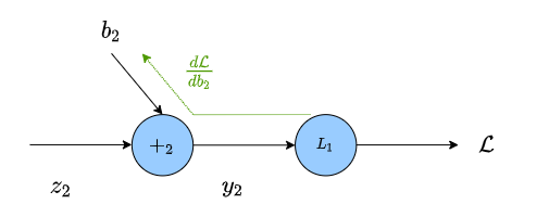
Lets first look at updating $b_2$ using the SGD updating scheme with learning rate $\eta$.
\[b_2 \leftarrow b_2 - \eta \frac{d\mathcal{L}}{db_2}\]To do this, we need to find $\frac{d\mathcal{L}}{db_2}$. This is our gradient.
As you can see in the graph, $\mathcal{L}$ isn’t directly a function of $b_2$.
Instead we have the sequence of equations
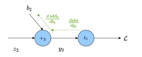
\[\begin{align} y_2 &= b_2 + z_2 \\ \mathcal{L} &= |y_2 - t| \end{align}\]To better visualize the gradients, we’ll rewrite our sequence of equations above in operator form:
\[\begin{align} y_2 &= {\rm add}(b_2, z_2) \\ \mathcal{L} &= {\rm abs}(y_2, t) \end{align}\]From this, we can see how the chain rule allows us to update $b$ based on $\mathcal{L}$
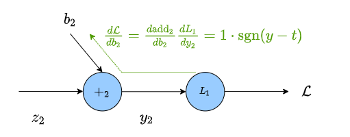
where $\frac{d}{db_2}{\small \rm add_2}$ is the derivative of the operation $(z_2 + b_2)$ w.r.t. $b_2$
\[\begin{align} &\frac{d}{db_2} (z_2 + b_2) = 1 \\ &\frac{d}{dy_2} {\rm abs}(y_2, t) = \text{sgn} (y_2-t) \end{align}\]The gradient is then the product of all of the edges between the weight we want to update and our loss
For the other values we keep doing the same thing,
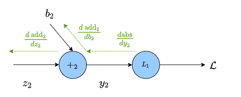
Once we’ve calculated the gradient at an edge, we don’t need to recalculate it. If we’re finding the gradients upstream, we only need to preform the chain run back to the previous calculation.
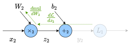
Where, in the above graph, we already know $\frac{d \mathcal{L}}{dz_2}$. such that
\[\begin{align} \frac{d \mathcal{L}}{dz_2} & = \frac{d{\rm add_2}}{dz_2}\frac{d {\rm abs}}{dy_2}\\ & = 1 \cdot \text{sgn} (y_2-t) \end{align}\]so we only need to calculate $\frac{d {\rm mul_2}}{dW_2}$.
\[\frac{d {\rm mul_2}}{dW_2} = x_2\]giving us our weight update term
\[W_2 \leftarrow W_2 - \eta \frac{d\mathcal{L}}{dW_2}\]wherein our gradient is:
\[\begin{align} \frac{d\mathcal{L}}{dW_2} &= \frac{d {\rm mul_2}}{dW_2}\frac{d \mathcal{L}}{dz_2} \\ &= x_2 \cdot 1 \cdot \text{sgn}(y_2-t) \end{align}\]The whole graph can be filled in like this.
If we were to write our own framework, we can put this into code by specifying the forward function, and the derivative of that function with respect to it’s inputs. The gradient we calculate from this is then passed to the parent operation to use in that calculation.
For example, the operation of a dot product might look like this:
class MatMul:
     def __init__(self, shape):
         self.w = np.random.rand(*shape)

     def forward(self, x):
         self.x = x
         return self.x @ self.w

     def backward(self, grad):
         self.dldw = self.x.T @ grad
         dldx = grad @ self.w.T
         return dldx

     def update(self, eta):
         self.w -= eta * self.dldw
where the derivatives are extended to support tensor values.
As Andre Karpathy said: yes, you should really understand backprop (which, btw, would be a really good article to read as a follow up). Hopefully this post has helped to make sense of this algorithm.
To continue to build intuition, it can be helpful to play around with an autograd framework (like pytorch). Try to use the code snippit below to answers some questions like:
- Why is it a bad idea to initialize all the weights in your network to 0?
- Is it a problem if you only initialize one set of weights in your network to 0
- The derivative of
reluis the Heavyside function. How might this lead to the dead neuron issue. How does leaky relu correct this?
>>> import torch
>>> import torch.nn as nn
>>> x = nn.parameter.Parameter(torch.randn(1,3))
>>> x.retain_grad()
>>> w = nn.parameter.Parameter(torch.randn(3,3))
>>> w.retain_grad()
>>> b = nn.parameter.Parameter(torch.randn(3))
>>> b.retain_grad()
>>> z = x @ w + b
>>> z.retain_grad()
>>> y = torch.relu(z)
>>> l = torch.sum(torch.abs(y))
>>> l.backward()
>>> z.grad  # inspect the gradient of an intermediate result
Of course, there’s no better substitute for learning this than building your own autograd framework. I recommend neural networks from scratch as a step-by-step guide to building your own “pytorch” or “tensorflow”.