ML Interview Prep: Linear Regression
Under construction
These posts are designed to be a quick overview of each machine learning model. The target audience is people with some ML background who want a quick reference or refresher. The following questions are compiled out of common things brought up in interviews.
- Top-level
- What is the high-level version, explain in layman’s terms
- What scenario should you use it in (classification vs regression, noisy data vs clean data)?
- What assumptions does the model make about the data?
- When does the model break/fail (adv & dis-advantages)? What are alternatives?
- A bit more detail
- How do you normalize the data for the model?
- What’s the loss function used?
- What’s the complexity?
- In-depth
- Probabilistic interpretation
- Derivation
- Simple implementation
- More on training the model
- How can you validate the model?
- How do you deal with over-fitting?
- How to deal with imbalanced data?
1. Top-level
1.1 High-level Explanation
Linear regression predicts a target value, $y$, given some input data, $x$.
\[y=wx+b\]The relationship between $y$ and $x$ is dictated by the proportionality factor $w$ (or ‘weight’) and the offset value, $b$ (otherwise called the ‘bias’). The goal in training a linear regression model is to find these coefficients, $w$ and $b$ [Goodfellow, Section 5.1.4].
A closed form solution exists to find these values; meaning, we can find $w$ and $b$ without the use of numerical tricks or iterative methods.
Consider the following simple example, lets say we have these three data points from the line $y=3x+1$:
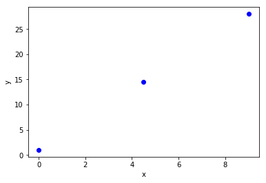
Our goal is to recapture the ground truth line of $y=3x+1$, using linear regression.
We can represent these data points in the following matrix form, such that each row is a data point pair ($x,y$-combination) and each column is the feature of interest:
\[\begin{align*} Y &= wX+b \\ \begin{bmatrix} 1 \\ 14.5 \\ 28 \end{bmatrix} &= \begin{bmatrix} 0 & 1 \\ 4.5 & 1 \\ 9 & 1 \end{bmatrix} \end{align*}\]Utilizing some matrix identities (discussed in section 3.2) we can find the weight matrix, $W$, with the following equation:
\[W= \left ( X^TX \right )^{-1} X^T Y\]X = np.array([
[ 0, 1],
[4.5, 1],
[ 9, 1]
])
Y = np.array([
[1 ],
[14.5],
[28 ]
])
W = np.linalg.inv( (X.T).dot(X) ).dot(X.T).dot(Y)
print("The equation for the line is y = {:.0f}x + {:.0f}".format(*W.flatten()))
The equation for the line is y = 3x + 1
In practice it can be impractical to obtain the answer from this analytic solution. Only in well-behaved scenarios is the matrix $X$ invertible, and, in cases where it is, this is extremely computationally expensive to do when $X$ is large. Moreover, $X^{-1}$ can only be represented to a limited precision on a digital computer, further introducing errors [Goodfellow Section 2.3]. Instead, methods like Generalized least squares are used; Or, we obtain the solution numerically using gradient decent (section 3.3).
1.2 What scenario should you use linear regression
Linear regression is an appropriate choice for predicting continuous target values, $y$, from continuous descriptive variables, $x_i$. It is commonly used in scenarios where the speed of predicting the target value is most desired attribute, and where less emphasis needs to be placed on accuracy of the prediction (the reason for this will be apparent in the next section).
1.3 Assumptions of Linear Regression
Linear regression works on the fundamental assumption that the predicted target value, $y$, is a linear combination of the descriptive values, $x_i$. Because of this, a significant amount of care needs to be taken in the construction of the model’s feature set (descriptive values).
An example of this is any prediction where the target is a direct linear combination of the descriptive values. Lets consider the case
\[y = w_1 x_1 + w_2 x_2.\]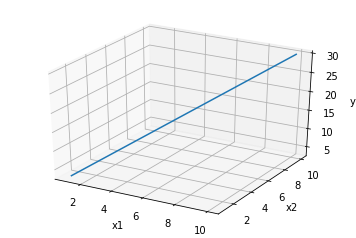
Where it should be obvious that $y$ is a linear combination of $x_i$.
A problem which might be less intuitive is the application of linear regression to finding the target values to a function of the form
\[y = w_1 x + w_2 x^2\]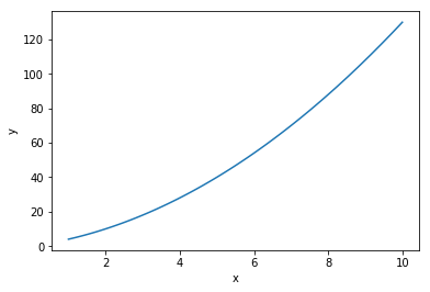
It might seem like this problem is non-linear; however, an important thing to remember is that linear regression only requires the problem to be linear w.r.t. the coefficients of the descriptive variables [James et al. Section 3.3.2]. To understand this, consider the above example, but rewritten as
\[\begin{align*} && y &= w_1 x + w_2 x^2 \\ && &= w_1 x_1 + w_2 x_2 \\ \text{with} && x_1 &= x \\ && x_2 &= x^2 \end{align*}\]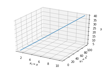
This shows that the non-linear term in $x$ can be treated as a separate feature. That is, by considering an extra dimension to the problem, we can map the non-linear behavior into a linear representation.
If the target values are not a linear combination w.r.t. the weights, such as
\[y = w^x\]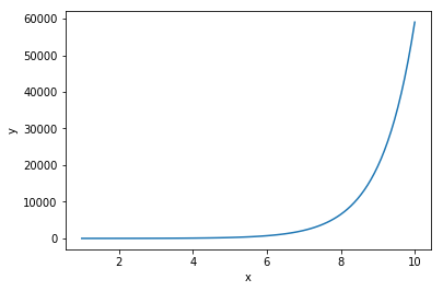
all hope is not lost. Consider a decomposition of the form
\[\log y = x \log w\]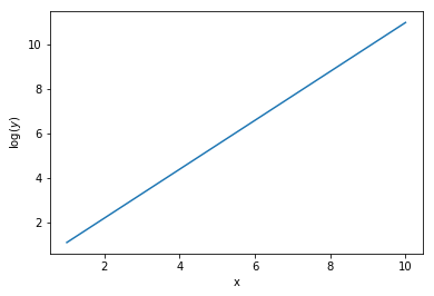
It should now be obvious that a significant amount of feature engineering is required to construct a linear regression model which accurately describes the target values. Doing this requires careful cleaning of the dataset and sufficient domain knowledge, such that the form of the equation is known a priori, and linear regression is only used to solve for the unknown dependencies, $w_i$.
1.4 When the model breaks & what’s a good backup?
If a linear dependence is not obtainable or if the appropriate equation can not be assumed, linear regression will fail. Depending on your application, you need to decide if the introduced errors from this are within your range of acceptability. If they are not, a new model will need to be implemented.
2. A bit more detail
2.1 Normalization of data
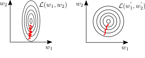
Although normalization is not strictly necessary for linear regression, properly scaling the feature variables can make a huge difference in the speed of convergence during the learning phase. Consider a dataset with two features which are of significantly different magnitude, for example predicting housing prices based on yard size and number of bedrooms in the house. The yard size could be of order 1000 ft² while the number of bedrooms might range from 0–5. While learning, slight variations in the weights of one feature can cause large swings in the error function. In this case, gradient decent will preferentially try to optimize to this variable. This can lead to oscillations in the loss-space, slowing down the rate of convergence (illustrated below) [Goodfellow et al. Section 4.3.1].
2.2 Loss function
2.2.1 Mean Squared Error (L2 loss)
The most commonly used error function for linear regression is the MSE:
\[\mathcal{L} = \sum^N_i \left ( XW - Y \right ) ^2\]This has the benefit that the solution is unique, and that the model can approach it stably. However, some drawback to it include its susceptibility to error due to placing heavy weight on any outlier data points.
2.2.2 Absolute Value (L1 loss)
Another loss function is the absolute value:
\[\mathcal{L} = \sum^N_i \left | XW - Y \right |\]This solution is not unique, due to the discontinuity in the derivative at $ Y=XW$; however, it often performs better in situations with more outliers [Murphy, Section 7.5].
2.3 What’s the complexity
training: $\mathcal{O}(p^2n+p^3) $
prediction: $\mathcal{O}(p)$
Wherein $n$ is the number of training sample and $p$ is the number of features [7]
3. In-depth
3.1 Probabilistic interpretation
We are trying to find the line, $\hat{y} = XW$, which maximizes the probability that a given point, $(y_i, x_i)$, from our dataset will fall on that line [Bishop Section 1.2.5].
To say that another way, “what is the probability that our best-fit-line is correct, given the data we have”. This is denoted mathematically as $P( \hat{y}_i | y_i)$.
From Bayes’ Law, we know the above relation can be described as
\[P(\hat{y}_i | y_i) = \frac{ P(\hat{y}_i) P(y_i|\hat{y}_i) }{P(y_i)}.\]To answer the above question, and find the best-fit-line, we need to maximize the likelihood, $P( y_i | \hat{y}_i )$, that a single data point, $y_i$, from our dataset will come from a distribution given by our best-fit-line, $\hat{y}_i$. It is our responsibility to select the distribution function that represents this likelihood.
It is commonly assumed that the noise, or scatter, in the observed data is due to random observational error [Bishop, Section 3.1.1]. If we make this assumption, it is acceptable to assume probability of a given value, $y_i$, would fall within a normal (Gaussian) distribution - where the value $\hat{y}_i$ is the mean of the distribution, $\mu$.
For a given input $x_i$ the likelihood of guessing the correct output is given as.
\[N_j(\mu, \sigma) = \frac{1}{\sqrt{2\pi \sigma^2}} \exp \left \{ - \frac{1}{2} \left ( \frac{y-\mu}{\sigma} \right )^2 \right \}.\]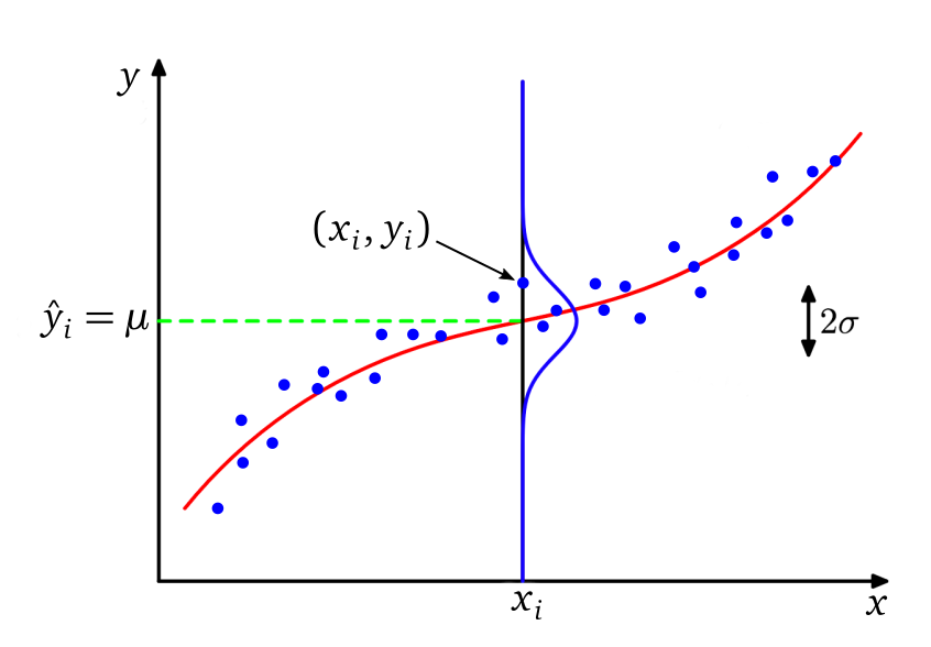
To calculate this efficiently when we extend to all input points $x_i$, we take the $\log$ of $P$; otherwise, we’ll be multiplying many numbers <1 together (if we don’t, we’ll end up with inaccuracies due to underflow) and also because it is less computationally expensive to compute [Murphy 3.5.3].
\[\log P = \sum_i \left [ -\frac{1}{2} \log (2\pi \sigma) - \frac{1}{2} \frac{(y_i - \mu_i)^2}{\sigma^2} \right ]\]And drop the constant terms:
\[\log P \propto -\sum_i \frac{(y_i-\mu_i)^2}{\sigma^2}.\]At this point, we’ve derived our L2 error function by showing that maximizing the log-likelihood is equivalent to minimizing the squared error [Murphy Section 7.3]:
\[\begin{align*} \log P &\propto -\sum_i (y_i-\mu_i)^2 \\ L_2 &= \sum_i (y_i-\hat{y}_i)^2 . \end{align*}\]Therefore, the using the mean-squared-error as a loss function is a direct consequence of assuming noise in the dataset is drawn from a Normal distribution [Bishop Section 1.2.5]. Similarly, if we had assumed a different likelihood distribution, such as a Laplace distribution:
\[P(y | \mu, b) = \frac{1}{2b} \exp \left \{ -\frac{\left | y - \mu \right |}{b} \right \}.\]Then we would have arrived at a different loss function. In the case of a Laplace distribution, this would be the L1 loss function [Murphy Section 7.4].
3.3 Derivations
3.3.1 Derivation of the analytic solution
We assume that the best fit line to the data will be one which minimizes the squared error. From calculus we know $\mathcal{L}$ will be at a minimum when $\frac{d}{dW} \mathcal{L}=0$
\[\begin{align*} \mathcal{L} &= (XW - Y)^T(XW-Y) \\ &= (XW)^T(XW) - (XW)^TY - Y^T(XW) + Y^TY \\ &= W^TX^TXW - 2(XW)^TY + Y^TY \\ \end{align*}\]taking the derivative and setting to zero
\[\frac{d}{dW}\mathcal{L} = 2X^TXW - 2X^TY = 0\]yields
\[X^TXW = X^TY. \\\]Such that
\[W = (X^TX)^{-1}X^TY.\]See this wikipedia page on linear regression estimation methods for other analytic solutions.
3.3.2 Derivation of gradient decent
In cases where it is infeasible to obtain the solution analytically, we find a solution numerically by iteratively converging on the condition $d\mathcal{L}/dw = 0$. We define this action as
\[w \leftarrow w - \eta \cdot \frac{d}{dw}\mathcal{L}\]Such that, at every iteration we update the weights with the R.H.S. When $d\mathcal{L}/dw = 0$, the weights will have converged to their optimal solution i.e. $w \leftarrow w$.
With our loss function defined as:
\[\mathcal{L} = \sum^N_i (w^Tx_i-y_i)^2\]we find the derivative w.r.t. the weights is
\[\frac{d}{dw}\mathcal{L} = \sum^N_i 2(w^Tx_i-y_i) x_i\]Using matrix notation and absorbing the 2 into the learning rate, $\eta$, we can then use the following equation to minimize the loss using gradient decent [Goodfellow, Section 5.9]
\[W \leftarrow W-\eta X^T (XW-Y)\]The learning-rate is a somewhat-arbitrary constant chosen to dictate the rate-of-convergence. However, care must be exercised in selecting this value. Too high of a learning rage can lead to divergence of the problem [learning-rate finder].
3.4 Simple implementation
class LinearRegression:

    def __init__(self, order):
        self.W = np.random.randn((order+1))

    def fit(self, X, Y, lr=1e-5, epochs=1000):
        X = np.vstack((X, np.ones_like(X))).T
        Y = Y.T

        for _ in range(epochs):
            err = self.perdict(X) - Y  # (Y_hat - Y)
            dL = X.T.dot(err)          # 2 X^T (Y_hat - Y), absorbing 2 into the learning rate
            self.W -= lr*dL         # W <- W - lr * dL/dW

    def perdict(self, X):
        return X.dot(self.W)

    def coeff(self):
        return self.W.ravel()


if __name__ == '__main__':

    x = np.linspace(0,25,100)
    epsilon = 3*np.random.randn(len(x))
    y = 3*x + 1 + epsilon

    lr = LinearRegression(order=1)
    lr.fit(x,y)
    w, b = lr.coeff()

    plt.plot(x, y, 'bo')
    plt.plot(x, w*x+b, 'r')
    plt.xlabel("x")
    plt.ylabel("y")
    plt.show()

    print(f"Equation of the line is y = {w:.0f}x + {b:.0f}")
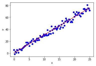
Equation of the line is y = 3x + 1
4. Training the model:
4.1 How can you validate the model?
4.2 How do you deal with over-fitting?
4.3 How to deal with imbalanced data?
5. References
The notes above have been compiled from a variety of sources:
- G. James, D. Witten, T. Hastie, and R. Tibshirani. An Introduction to Statistical Learning. Springer, 2017.
- C. M. Bishop. Pattern Recognition and Machine Learning. Springer, 2011.
- K. P. Murphy. Machine Learning: A Probabilistic Perspective. The MIT Press, 2012.
- T. Hastie, R. Tibshirani, and J. Friedman. The Elements of Statistical Learning, Second Edition. Springer, 2016.
- I. Goodfellow, Y. Bengio, and A. Courville. Deep Learning. MIT Press, 2016.
- A. Ng, CS229 Lecture notes, 2018
- Computational complexity learning algorithms, 2018