ML Interview Prep: Logistic Regression

Under construction

These posts are designed to be a quick overview of each machine learning model. The target audience is people with some ML background who want a quick reference or refresher. The following questions are compiled out of common things brought up in interviews.

Top-level
1. What is the high-level version, explain in layman’s terms
2. What scenario should you use it in (classification vs regression, noisy data vs clean data)?
3. What assumptions does the model make about the data?
4. When does the model break/fail (adv & dis-advantages)? What are alternatives?
A bit more detail
1. How do you normalize the data for the model?
2. What’s the loss function used?
3. What’s the complexity?
In-depth
1. Probabilistic interpretation
2. Derivation
3. Simple implementation
More on training the model
1. How can you validate the model?
2. How do you deal with over-fitting?
3. How to deal with imbalanced data?

1. Top-level

1.1 High-level explanation

Logistic regression is a machine learning model for classification, most commonly used for binary classification. The model can be extended to multi-class classification; however, in practice, other approaches are considered more favorable for this task. [James et al. Section 4.3.5]. In this post, we will only discuss the mechanics for binary classification.

Logistic regression finds a line-of-separation, otherwise called a ‘decision boundary’, representing the separation in classes describing the given input features.

It is defined by the functional form:

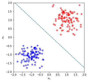
\[\begin{align*} y = f(x_1, x_2,\cdots, x_N) &= \sigma \left (\sum_i^N w_i x_i+b \right ) \\ &= \frac{1}{1+\exp\left\{ -(x^Tw+b) \right \}}. \end{align*}\]

Consider the example below, of two Gaussian clouds centered at (1,1) and (-1,-1):

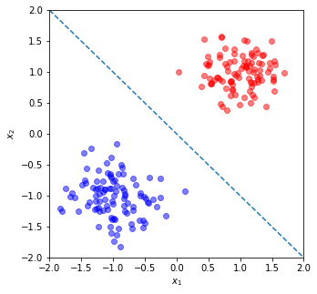
It should be obvious that the dashed dividing line, $x_2=-x_1$, separates the two classes, but lets explore this mathematically.

For the sake of this example, we’ll drop the sigmoid from the equation above. Using this, we can describe the system as:

\[f(x_1, x_2) = x_2 + x_1 = 0\]

Where we get $w_1=1$ and $w_2=1$ from the dividing line $x_2=-x_1$ (we know this a priori in this example). We now have the following relationship:

\[f(x, x) = \left\{\begin{matrix} {\rm Blue} & {\rm if } < 0 \\ {\rm Red} & {\rm if } > 0 \\ \end{matrix}\right.\]

Taking the center point of one of the Gaussian clouds, $(-1,-1)$, and plugging it in to the above equation yields:

\[\begin{align*} f(-1,-1) &= -2\\ -2 < 0 \therefore (-1,-1) &= {\rm Blue}. \end{align*}\]

Whereas, the point (1,1) yields:

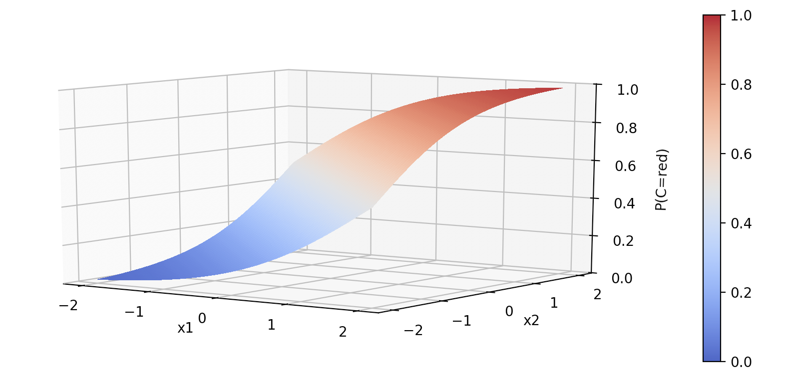
\[\begin{align*} f(1,1) &= 2 \\ 2 >0 \therefore (1,1) &= {\rm Red}. \end{align*}\]

Now, the values 2 or -2 are not particularly illuminating. So, we use the sigmoid function to squash the output into a probability [Murphy, Section 1.4.6], such that the output $y<.5\equiv{\rm Blue}$ and $y>.5\equiv{\rm Red}$. To put this graphically:

1.2 What scenario should you use logistic regression?

Logistic regression models are used mostly as a data analysis and inference tool, where the goal is to understand the role of the input variables in explaining the outcome. [Hastie et al. Section 4.4.1]

1.3 Assumptions of linear regression

The approach makes the explicit assumption that your data can be separated by a line or hyper-plane. Like linear regression, logistic regression is a linear model [Murphy, Section 1.4.6].

Therefore, logistic regression is an appropriate choice when classifying data that is linearly separable. This either has to be innately true or carefully constructed into custom ‘features’ - using sufficient domain knowledge. For example, consider the “donut” problem below:

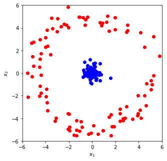
This is not a linear classification problem - no straight line will separate these classes. However, similar to the polynomial problem in my post on linear regression, we can construct a custom representation of the data by adding an extra dimension:

\[x_3 = \sqrt{x_2^2 + x_1^2}\]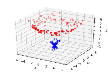

These clusters can now be separated with a hyperplane in $(x_1, x_2)$-space, at $x_3 \approx 2$.

1.4 When the model breaks & what’s a good backup?

The model will break when there is not a linear decision boundary the separates the two classes [Murphy, Section 1.4.6]. Depending on the requirements of the problem goal, different methods may be implemented based on a speed-accuracy-and-explainability trade-off.

2. A bit more detail

2.1 Normalization of data

Like Linear regression, normalization is not strictly necessary for logistic regression; however, properly scaling the feature variables can make a huge difference in the speed of convergence during the learning phase. This is because slight variations in the weights of one feature can cause large swings in the error function. In this case, gradient decent will preferentially try to optimize to this variable, leading to oscillations in the loss-space and slowing down the rate of convergence (illustrated below) [Goodfellow et al. Section 4.3.1].

2.1 Loss function

The loss function for binary logistic regression is the cross-entropy error

\[\mathcal{L} = - \left \{ t\log(y) + (1-t)\log(1-y) \right \}\]

wherein $t$ is the target class, and $y$ is the class predicted by the model.

It can be helpful to notice that only one of these terms will matter at a time. For example given a target class of $t=0$ only the second term will matter, $-\log(1-y)$. Whereas if $t=1$ only the first term will matter, $-\log(y)$.

2.3 What’s the complexity

The complexity for logistic regression is the same as for linear regression:

training: $\mathcal{O}(p^2n+p^3) $
prediction: $\mathcal{O}(p)$

Wherein $n$ is the number of training sample and $p$ is the number of features [8]

3. In-depth

3.1 Probabilistic interpretation

Logistic regression operates on the fundamental assumption that the data falls into a binomial distribution and that each of the data points are independent from one-another.

We approach this derivation this using Bayes’ Law. For a justification of the Bayesian approach, check out the probablistic interpretation section, 3.1, of my post on linear regression.

To learn the system, we want to maximize the probability that we correctly predict the correct answer $\hat{Y},$ determined by the equation $\hat{Y} = \sigma \left ( WX \right )$, given our input features $X$ and the true class values $T$. i.e. we want to maximize $ P(\hat{Y}|X, T).$ This is equivalent to saying, “we want to maximise the probability that the weights are correct, given our inputs and class labels, $P(W | X, T)$. Using Bayes rule, we can now write:

\[P(W | X, T) = \frac{P(T | W, X) P(W)}{P(T)}\]

We assume all weights are equally likely and the dataset is balanced, therefore the term in this that we have control over is the likelihood, $P(T |W, X)$ [Bishop, Section 4.3.2]. We want to maximize this term during training, thereby maximizing the probability that the data points, $X$, fall into the correct class for a given weight configuration, $W$, $P(T|W,X)$.

We define the likelihood based on out prior belief that the data will fall into a binomial distribution.

\[\begin{align*} P(T | W) &= P(t_1, t_2, \cdots, t_N | W) \\ &= \prod_{i}^{N} P(t_i | W) \\ &= \prod_{i}^{N} \hat{y}_i^{t_i}(1-\hat{y}_i)^{1-t_i} \end{align*}\]

Taking the negative log of this, to avoid multiply small numbers together and to reduce the complexity of calculating exponents, renders the cross-entropy loss function.

\[- \log P(X|y) = \sum_i \left \{ t_i\log y_i + (1-t_i)\log (1-y_i) \right \}\]

Where $\hat{y_i} = P(C | W, x_i) = \sigma (Wx_i)$.

To summarize, logistic regression fundamentally assumes the data falls into a binomial distribution, and by maximizing the log of the likelihood (log-likelihood) we minimizing the cross-entropy error [Bishop, Section 4.3.2].

3.2 Derivations

3.2.1 Closed-form solution

Unlike Linear Regression, we cannot write a general closed-form solution to logistic regression [Bishop, Section 4.3.3].

3.2.2 Numerical solution

We can use gradient decent,

\[w \leftarrow w - \eta \frac{d}{dw}\mathcal{L},\]

to find the solution numerically [Hastie et al. Section 4.4.1].

With our definition of loss being the cross-entropy, we find it’s derivative with-respect-to the model weights using the chain rule:

\[\frac{d}{dw}\mathcal{L} = \frac{d\mathcal{L}}{dy}\frac{dy}{dz}\frac{dz}{dw}\]

where

\[\begin{align*} y &= \sigma(z) \\ z &= w^Tx \\ \\[5mm] \end{align*}\]

We then find the derivatives of each component:

\[\begin{align*} \frac{d\mathcal{L}}{dy} &= -\frac{d}{dy} \sum_i \left \{ t_i\log(y_i) + (1-t_i)\log(1-y_i) \right \} \\ &= - t\frac{1}{y_i} - (1-t_i)\frac{1}{1-y_i}, \\ \\[2mm] \frac{dy}{dz} &= \frac{d}{dz} \frac{1}{1+\exp(-z)} \\ &= \frac{1}{1+\exp(-z)}\frac{\exp(-z)}{1+\exp(-z)} \\ &= y(1-y), \\ \\[2mm] \frac{dz}{dw} &= \frac{d}{dw} w^Tx \\ &= x. \end{align*}\]

Rendering,

\[\begin{align*} \frac{d}{dw}\mathcal{L} = \sum_i (y_i-t_i)x \end{align*}\]

3.3 Simple Implementation

class LogisticRegression:

    def __init__(self, order):
        self.W = np.random.randn((order+1))

    def fit(self, X, Y, lr=1e-1, epochs=1000):
        N, D = X.shape
        X = np.hstack((X, np.ones(shape=(N,1))))

        for _ in range(epochs):
            Y_hat = self.perdict(X)
            dL = X.T.dot(Y_hat-Y)  # X^T (Y_hat - Y)
            self.W -= lr*dL

    def perdict(self, X):
        return 1/(1+np.exp(-X.dot(self.W)))

    def coeff(self):
        return self.W.flatten()


def generate_data():
    X = np.random.randn(200,2)/3
    X[100:,:] += 1
    X[:100,:] -= 1
    Y = np.zeros(200)
    Y[100:] = 1

    plt.figure(figsize=(5,5))
    plt.scatter(X[Y==0,0], X[Y==0,1], color='b', alpha=.5)
    plt.scatter(X[Y==1,0], X[Y==1,1], color='r', alpha=.5)
    plt.xlabel("$x_1$")
    plt.ylabel("$x_2$")
    plt.xlim(-2,2)
    plt.ylim(-2,2)
    plt.show()

    return X, Y


X, Y = generate_data()

lr = LogisticRegression(order=2)
lr.fit(X, Y)

w1, w2, b = lr.coeff()

x = np.linspace(-2, 2, 100)
m = -w1/w2
b = (b-.5)/w2
y = m*x + b

print(f"The decision boundary is along: x2 = {m:.0f}x1 + {b:.0f}")
plt.plot(x, y, '--')

The decision boundary is along: x2 = -1x1 + 0

4. Training the model:

4.1 How can you validate the model?

4.2 How do you deal with over-fitting?

4.3 How to deal with imbalanced data?

5. References

These notes above have been compiled from a variety of sources: