ML Interview Prep: Naive Bayes
These posts are designed to be a quick overview of each machine learning model. The target audience is people with some ML background who want a quick reference or refresher. The following questions are compiled out of common things brought up in interviews.
- Top-level
- What is the high-level version, explain in layman’s terms
- What scenario should you use it in (classification vs regression, noisy data vs clean data)?
- What assumptions does the model make about the data?
- When does the model break/fail (adv & dis-advantages)? What are alternatives?
- A bit more detail
- How do you normalize the data for the model?
- What’s the complexity?
- In-depth
- Probabilistic interpretation
- Derivation
- Simple implementation
- More on training the model
- How can you validate the model?
- How do you deal with over-fitting?
- How to deal with imbalanced data?
1. Top-level
1.1 High-level Explanation
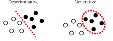
Naive Bayes is a generative model for classification. Generative models are ‘generative’ because they explicit specify the likelihood of the data and the probability of class occurrence. Generative models differ from discriminative models which find a hard decision boundary - separating the target classes - by directly fitting the class posterior [Murphy. 2.2.3.2]. Examples of discriminative models would be logistic regression or Decision Trees.
Unsurprisingly, Naive Bayes is governed by Bayes’ Law, under the assumption that all data is conditionally independent [Murphy 3.5; V. Lavrenko; Pang-ning 5.3.3]:
\[\underbrace{P(Y|X)}_{\rm posterior} = \frac{\overbrace{P(X|Y)}^{\rm likelihood} \overbrace{P(Y)}^{\rm prior}}{\underbrace{P(X)}_\text{probability of seeing the data}}.\]Our goal is to obtain an understanding of the probability that a given selection of data, $X$, will indicate the presence of a class $Y$, i.e. $P(Y|X)$. Our ability to find this relation depends on our prior belief about how probable it is for class $Y$ to occur, $P(Y)$; the likelihood that we will see that set of data, $X$, given occurrence of class $Y$, $P(X|Y)$; and the overall probability of seeing the data in the first place, $P(X)$.
This is easier to understand with an example:
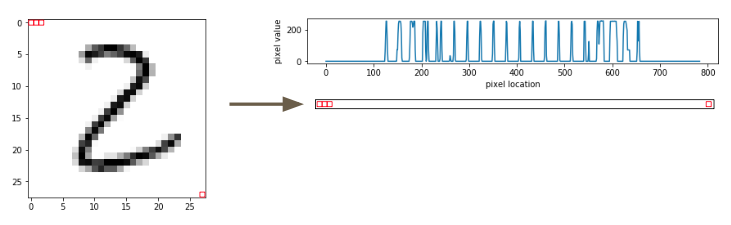
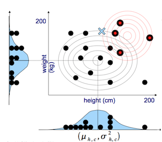
Let’s consider a Naive Bayes approach to the MNIST dataset. We select an image of the number ‘two’ and flatten it to a vector. We then plot the intensity for each pixel vs. the pixel number.
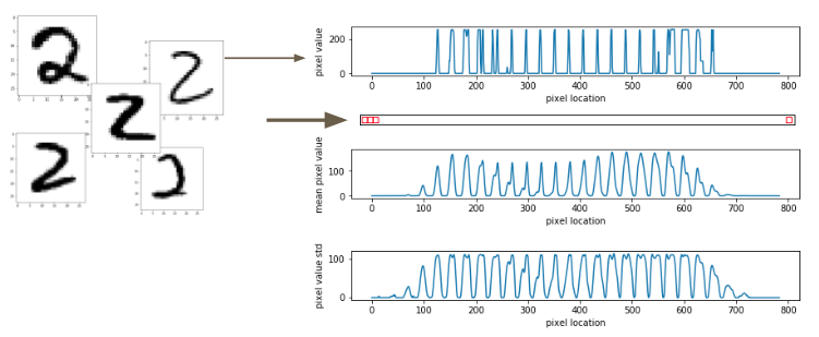
We can do this for every ‘two’ and build up an understanding of the average intensity at each pixel (mean, $\mu$), as well as what pixels see the widest variety of intensities (standard deviation, $\sigma$).
We now have to make an explicit assumption about the probability distribution we expect the data to fall into. For this we have two options:
- Build it using the maximum likelihood procedure [Murphy 3.5.1.1]
- We can assume a PDF [Pang-ning 5.3.3]
Your choice for these options will depend on if your data is continuous or discrete, and, if discrete, how sparse the data is. For this example, we will assume Gaussian normal PDF for the likelihood, but we will discuss the Pros and Cons later.
Now that we have our PDF function, we can generate a probability map based on the two parameters that describe it, $\mu$ and $\sigma$. We do this for all other classes (numbers) in the dataset.
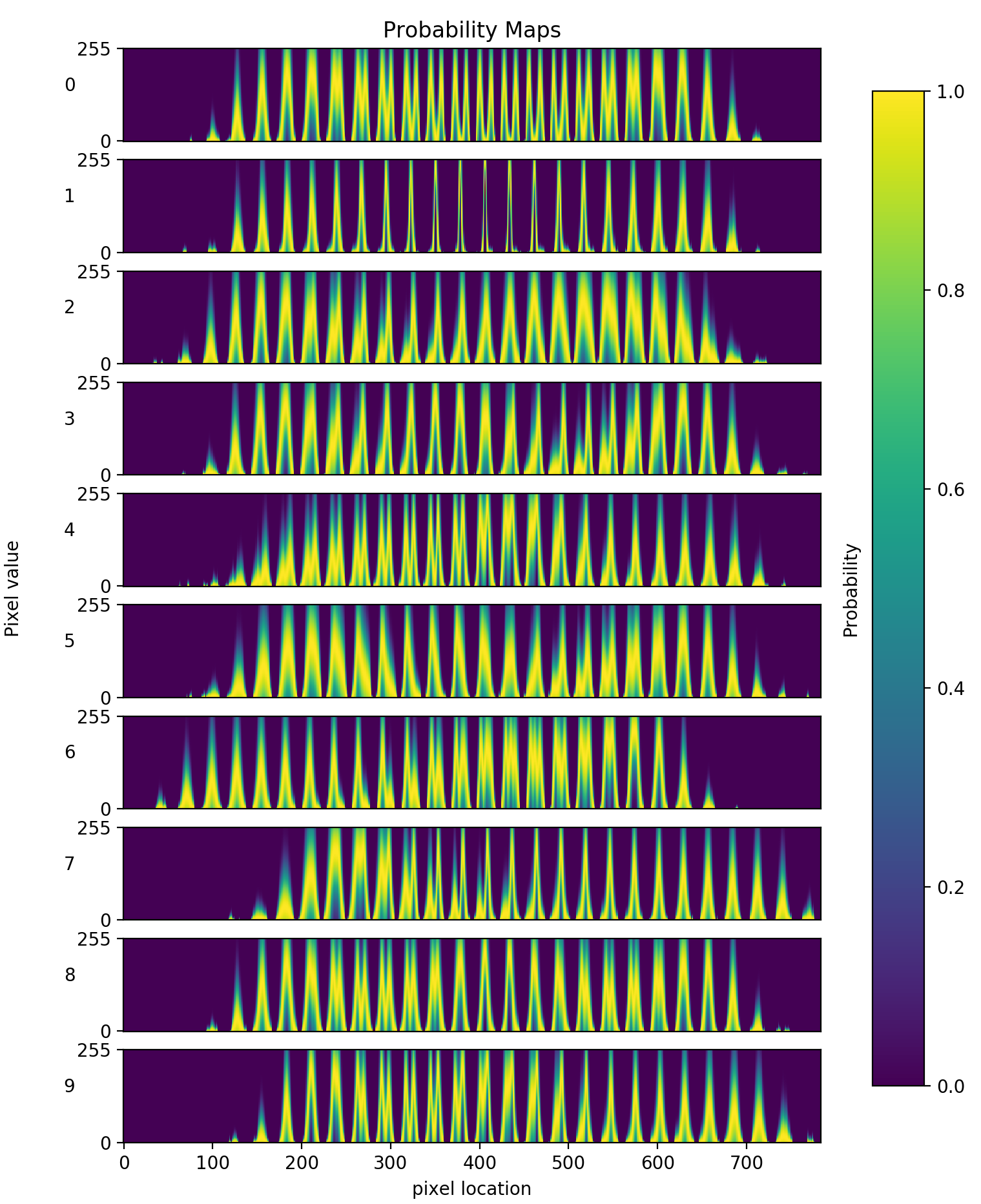
Each of these probability maps acts as a thumb-print to describe a class. Mathematically, we’ve built up the probability of seeing a set of features (pixel intensities) given a class,
\[P(X|Y).\]This is defined as the likelihood, e.g. What is the likelihood that a select pixel will have a value of 255 given the digit is a 2.
Next, we encode our prior knowledge about the occurrence of the classes $Y$. For digits, we’ll say all values $\{0, \cdots, 9\}$ are equally likely. i.e. $P(Y) = 1/10$. However, if we knew this was not the case we can encode this information as well. As a trivial example: if we knew we were classifying binary values we would set $P(Y{=}0) = P(Y{=}1) = .5$ and $P(Y{=}2, \cdots, 9) = 0$.
Now, if all were doing is picking the most likely class, we can drop the denominator $P(X)$. This is the overall probability of seeing the data and only serves as a normalization constant; so, it will be constant for each class. We can drop it and still obtain the most likely class:
\[\begin{align*} \hat{y} &= \arg \max_i \left \{ P(Y{=}y_i | X) \right \} \\ &= \arg \max_i \left \{ P(X | Y{=}y_i) P(Y{=}y_i) \right \}. \end{align*}\]If we want the true probability, then we have to calculate $P(X)$
\[P(X) = \sum_{i} P(X|Y{=}y_i)P(Y{=}y_i)\]1.2 What scenario should you use it in?
Ideally, Naive Bayes should only be used in scenarios when the “naive bayes assumption” is true. That is, when the data are conditionally independent from one-another:
\[P(X|Y{=}y) = \prod_i^d P(x_i|Y{=}y)\]However, even in scenarios where the naive assumption is not true, the NB classifier can still out perform other models [Murphy 3.5; Hastie 6.6.3].
Some instances where you see Naive Bayes commonly used are in scenarios where the datasets contains noisy data, missing data, a class imbalance, or when the dataset is small and the dimensionality is large. This is assuming one knows an accurate model for the prior and likelihood distributions (see below for discussion).
1.2.2 Noisy data
NB is well equipped to handle noisy data. Consider the example of an email spam detector. Background noise might be stop words, like “the”, “is”, “and”, “at”, or “which”. In our spam/not-spam classifier for emails, these words would show up with the same regularity in each classification model. That is, the likelihood of seeing “the” is the same for an email that is spam and one that is not spam:
\[P( X{=}\text{the} \,|\, \text{spam} ) = P( X{=}\text{the} \, | \, \neg \text{spam} ).\]In this case, the likelihood for spam/not-spam would both increase by the same constant, making this feature irrelevant for the classification decision. So, we don’t need to clean these features from our dataset [T. Pang-Ning, 5.3.3].
1.2.3 Missing values
Naive Bayes is very capable of handling missing values during inference. In this case, only the likelihoods based on the observed values are calculated [V. Lavrenko IAML5.14].
\[P(x_1 + \cdots + x_j + \cdots + x_d | y) = \prod^d_{i \neq j} P(x_i | y)\]Wherein $x_j$ is a value missing during inference.
1.2.4 Minority Class
The dataset does not need to be balanced during training. Unlike a discriminative model (which is trained to directly predict the posterior; and, therefore, implicitly assumes the probability of class occurrences, NB requires an explicit description of the class occurrence [Citation needed].
1.2.5 Small datasets
Naive Bayes is a popular choice when density estimation methods are not appropriate, such as when the dimensionality of the data is high and the dataset is small [Hastie 6.6.3]. The model only has $\mathcal{O}(CD)$ parameters - in the MNIST example we had C=10 (digits) and D=2 ($\mu$ and $\sigma$). The simplicity of this model makes it relatively immune to overfitting [Murphy 3.5].
1.3 What assumptions does the model make about the data?
As stated above, NB makes the fundamental assumption that the data points are conditionally independent given the class label [Murphy, 3.5; Pang-Ning, 5.3.3]:
Additionally, if the data is continuous or too space, such that the MLE method for generating likelihood cannot be used, then a PDF must be assumed. In the example below, NB will classify the data as described by a Normal distribution. It will make this assumption even if the sample histogram does not immediately mimic the assumed PDF [Lavrenko, Naive Bayes 3].
1.4 When does the model break / fail?
Naive Bayes can fail when independence between input features is not true. When Google was first rolling out their search engine, Naive Bayes was used on the back-end to make predictions [Malone, Lesson 2]. They ran into issues when people wanted to search for things like “the Chicago Bulls;” the Naive Bayes model classified this as a ‘location’ and an ‘animal.’ However, we know from context that this is neither of these things, the query should instead be classified as ‘basketball team’.
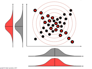
1.4.1 Correlated attributes
Another failure point with Naive Bayes is its inability to separate classes when the only thing distinguishing them is their correlation. Because it is making the naive assumption, it cannot distinguish between the two examples in the below image - as the probability distributions are completely overlapped [Lavrenko IAML5.11]
1.4.2 Zero-frequency occurrence / Black swan paradox
If an MLE approach is use with Naive Bayes, then the implementer needs to be careful about handling rare-events. Because the finally probability is a function of the products of the likelihoods, an occurrence that has been seen for one class but never been seen for another (lets say $x_j$) will generate a probability of 0 for the second class. This is an unrealistic assumption, to base your entire prediction on the occurrence of one data point.
\[P(x_1 + \cdots + x_j + \cdots + x_d | y) = P(x_1|y) \times \cdots \times \underbrace{P(x_j|y)}_0 \times \cdots \times P(x_d|y)\]This is typically combatted using Laplace smoothing [Murphy 3.4.1.2; Lavrenko IAML5.13]. Effectively, a small number is added to every probability to ensure there is never a multiplication by zero.
1.4.3 What to use when it fails
2. A bit more detail
2.1 How do you normalize the data for the model, if you need to?
Although it is not strictly necessary to normalize the data going into a NB classifier, not doing so can add unnecessary complexity [citation needed]:
During the training of the model, a small number, $\epsilon$, is added to the standard deviation as a smoothing parameter to avoid division by zero. i.e. $ \exp \{ (\mu-x)^2 / 2(\sigma + \epsilon)^2 \}$
If the features, $x$, vary in range, then the smoothing parameter would have to change to reflect this. This value can have a significant effect on the accuracy of the model. To convince yourself of this, try changing $\epsilon$ in the code below.
2.2 What’s the complexity?
NB is one of the fastest learning methods.
For number of classes $c$, number of instances $n$, number of dimensions $d$, the time complexity at training will be of order [Murphy 3.5.1.1]:
\[\mathcal{O}(nd+cd) \approx \mathcal{O}(nd)\]For a single input at inference, the complexity is [Murphy 3.5]
\[\mathcal{O}(dc)\]3. In-depth
3.1 Probabilistic Interpretation
The model assumes that the features, $X$, are conditionally independent from one another. For example, in a data set it might appear that there is a correlation between the occurrences of $B$ and $C$. However, if it can be assumed that $B$ and $C$ are actually mutually independent and the correlation can be attributed to the existence of an external factor, $A$, then we can apply Naive Bayes.

As an example: if one were to look at the rate of heat stroke and the action of going to the beach, there might be a correlation. However, there is nothing intrinsic about going to the beach that causes heat stroke. So, if we consider an external factor, the temperature, we can model these features as mutually independent. Such that, you’re more likely to go to the beach when its hot and your more likely to get heatstroke when its hot [V. Lavrenko Naive Bayes 2]. In a NB classifier, the predicted class is this hidden dependence. Such that:
\[P(Y{=}A | x_1{=}B, x_2{=}C)\]3.2 Derivation
The probability of a event $A$ and $B$ occurring, with the Naive Bayes assumption, is
\[P(A \cap B) = P(A|B)P(A).\]Likewise, the probability of an event $B$ and $A$ occurring is
\[P(B \cap A) = P(B|A)P(B).\]Because $P(A \cap B) == P(B \cap A)$ we can set the two equations equal to each other and find a description for the probability of $A$ occurring, given $B$ occurring:
\[P(A|B) = \cfrac{P(B|A)P(B)}{P(A)}.\]I don’t find the terms $A$ and $B$ particularly illuminating, so we can rewrite this in the Diachronic form: describing the probability of a hypothesis, $H$, being true, given some observations (or evidence), $E$, existing.
\[P(H|E) = \cfrac{P(E|H)P(H)}{P(E)}.\]Furthermore, the probability of an event, $P(E)$, is not always intuitively clear. I believe is it more obvious to write this in terms of $P(E)$ as a normalization constant:
\[P(H|E) = \cfrac{P(E|H)P(H)}{\sum_{H'} P(E|H')P(H')}.\]If we are only concerned with “What is the most probably hypothesis that describes evidence $E$”, we can drop the normalization (it is constant across all predictions). When we calculate these in practice, we take the log of the probabilities. This avoids underflow, due to taking the product of many numbers less than 1 [Murphy 3.5.3].
\[\hat{y} = \arg \max_i \left \{ \log P(y_i | X) \right \}\]such that
\[\log P(y_i | X) \propto \log P(X|y_i) + \log P(y_i)\]and $\hat{y}$ is equal to the most likely hypothesis for multiple evidence, $X$.
3.3 Simple Implementation
import numpy as np
from scipy.stats import norm
from sklearn.datasets import fetch_openml
from sklearn.model_selection import train_test_split


class NaiveBayes:

    def __init__(self):
        self.params = {}

    def fit(self, X, Y, epsilon=1e-2):
        """Fit NB classifier assuming a normal pdf for the likelihood

        Parameters
        ----------
        X : numpy.ndarray
            Training features. For MNIST, this is the pixel values
        Y : numpy.ndarray
            Target labels. For MNIST, this is the digits
        """
        for class_ in np.unique(Y):
            x_c = X[Y==class_]

            self.params[class_] = {
                'means': x_c.mean(axis=0),
                'std': x_c.std(axis=0) + epsilon,
                'prior': (Y==class_).mean(keepdims=True),
            }

    def predict(self, X):
        """Run inference on data

        Parameters
        ----------
        X : numpy.ndarray
            Data to predict on. dims 2: [number of cases, number of features]
        """
        N, _ = X.shape
        num_classes = len(self.params)
        log_posterior = np.zeros((N, num_classes))  # placeholder, we want to predict a class for each case

        # Calculate log P(Y|Y) = sum_i{log P(x_i|Y)} + log P(Y)
        # We do this for all cases simultaneously
        for class_, pram in self.params.items():
            log_liklehood = norm.logpdf(X, loc=pram['means'], scale=pram['std']).sum(axis=1)
            log_prior = np.log(pram['prior'])
            log_posterior[:, class_] = log_liklehood + log_prior

        return np.argmax(log_posterior, axis=1)

    def evaluate(self, X, Y):
        P = self.predict(X)
        return np.mean(Y == P)


print("Loading data... ")
X, Y = fetch_openml('mnist_784', version=1, return_X_y=True)
Y = Y.astype(int)
print("Done")

# Normalize with min-max scaling.
# The data does not need to be normalized; however, the smoothing parameter
# in training will have to change to compensate for this. If not normalizing,
# try epsilon = 255
X = (X - X.min()) / (X.max() - X.min())

xtrain, xtest, ytrain, ytest = train_test_split(X, Y)

nb = NaiveBayes()
nb.fit(xtrain, ytrain)
print("Accuracy on MNIST classification: {:.2f}%".format(100*nb.evaluate(xtest, ytest)))
Accuracy on MNIST classification: 70.38%
4. More on training the model
4.1 How can you validate the model?
NB can be evaluated use the common metrics: accuracy, F1, precision, recall. It’s important to evaluate the classifier in the context of the prior. That is, if you have a binary classifier with accuracy of 95% but the class occurrence in your dataset is 100:1, then your model may not be performing well.
4.2 How do you deal with over-fitting?
Naive bays is a high-bias model, as it only has a few parameters, $\mathcal{O}(dc)$. For the most part, this makes it relatively immune to overfitting [Murphy, 3.5]. However, the method in which NB is trained will effect is susceptibility to overfit. If the model is trained with a maximum likelihood procedure, then the likelihood is generated directly from the occurrences in the data. This can then creates the zero-frequency problem, discussed above. Under these circumstances, a distribution for the likelihood must be assumed, or, a strategy such as Laplace smoothing can be used [Murphy 3.4.1.2].
4.3 How to deal with imbalanced data?
Discussed in section 1.2.5 - Minority Class
5. References
- K. P. Murphy. Machine Learning: A Probabilistic Perspective. The MIT Press, 2012.
- V. Lavrenko. Naive Bayes Classifier, 2015
- T. Pang-Ning. Introduction to data mining. 2005.
- T. Hastie, R. Tibshirani, and J. Friedman. The Elements of Statistical Learning, Second Edition. Springer, 2016.
- K. Malone and S. Thrun. Intro to Machine Learning. Udacity, accessed: 6/2019